A weakly penalized discontinuous Galerkin method for radiation in dense, scattering media
Abstract
We review the derivation of weakly penalized discontinuous Galerkin methods for scattering dominated radiation transport and extend the asymptotic analysis to nonisotropic scattering. We focus on the influence of the penalty parameter on the edges and derive a new penalty for interior edges and boundary fluxes. We study how the choice of the penalty parameters influences discretization accuracy and solver speed.1. Introduction
The present paper reviews recent advances in discontinuous Galerkin (DG) methods for radiation transport in dense, scattering media and shows extensions to improve the boundary approximation and behavioral studies for nonisotropic scattering. Its focus is as in [14, 34], on the reliable discretization and efficient multigrid solvers in regimes where the mesh size of the discretization is considerably greater than the mean free path. It has already been observed in [1, 25] that the upwind DG method [26, 18, 35] suffers from loss of approximation in such regimes. This is exemplified in the top row of Figure 1 , where a simple model problem was solved with this method and the solutions converge to zero in an nonphysical way.
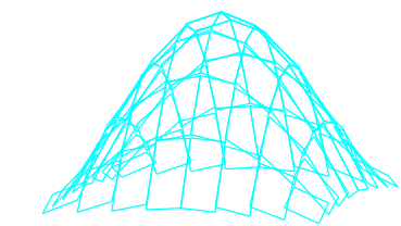
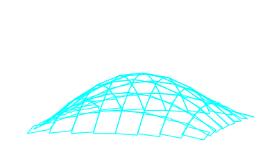
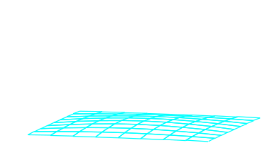
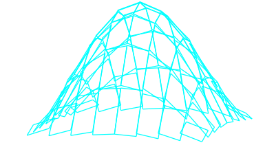
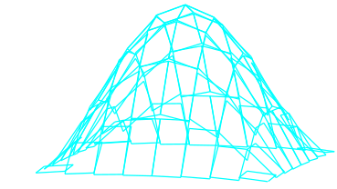
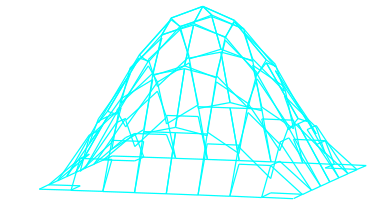
The mechanism behind this loss was analyzed in [1, 14] and a new, robust DG scheme (referred to below as RGK) was proposed by Ragusa, Guermond, and Kanschat in [34]. As it is seen in the second row of Figure 1, it has the correct convergence behavior. This scheme was improved and an efficient multigrid method was proposed in [22]. In both publications [22, 34] the DG method was not modified at the boundary. Analysis and numerical tests were confined to isotropic scattering.
We proceed as follows: in the following section we review the linear Boltzmann equation of monochromatic radiation transport and the asymptotic analysis leading to its diffusion limit. In Section 3, we derive the asymptotic expansion of the DG discretization and discuss an improved boundary model in 3.4. In Section 4, we review the derivation of an efficient multilevel Schwarz method and demonstrate its performance with the new boundary fluxes and for nonisotropic scattering.
2. Model and diffusion limit
We are considering radiation as a thin gas of small particles reacting with a background material but not with each other. Similarly to a Brownian motion process, a particle travels with constant momentum until one of the following events happens.- After an average distance of $1/{\widetilde\sigma_a}$ (the mean free path of absorption) since the last event, the particle is absorbed by the background and removed from the system.
- After an average distance of $1/{\widetilde\sigma_s}$ (the mean free path of scattering) the particle is scattered by a background particle, changing its momentum and continuing its journey with a new momentum.
The smallness assumption on the particles must be understood as the particle size being much smaller than either mean free path. For photons, this means that the wave length is negligible compared to these lengths. In addition, we make the modeling assumption that particles behave randomly. This implies small coherence length of optical radiation and in particular excludes lasers. Under this assumption, the motion of a sufficiently large sample of particles can be described by a linear form of the Boltzmann equation [8, 10, 27, 28] .
The basic quantity of radiation is a normalized density distribution function $\psi(\vx,\vO)$ of particles in phase space. We focus on photons here, such that the momentum space of $\R^d$ reduces to the sphere $S^{d-1}$ in dimensionless form. We obtain the equation \begin{align} \label{eq:1} \begin{aligned} \D\vO \psi(\vx,\vO) + \widetilde{\sigma}_a(\vx) \psi(\vx,\vO) + \widetilde{\sigma}_s(\vx) \Sigma \psi(\vx,\vO) = \widetilde q(\vx), \end{aligned} \end{align} where \begin{gather} \label{eq:paper:12} \Sigma \psi(\vx,\vO) = \psi(\vx,\vO)- \int_{S^{d-1}} H(\vO',\vO)\psi(\vx,\vO')\dO', \end{gather} with a scattering kernel $H(\vO',\vO)$ to be discussed below, see equations \eqref{eq:paper:13}--\eqref{eq:paper:15}.
Originally, this equation is posed on the whole of $\R^d$. Artificial boundaries can be introduced to form a bounded domain of interest $\Do$ for physical and numerical reasons, for instance if no radiation enters the domain of interest from the other side of such a boundary. Let $\vn_\Do$ be the outer unit normal vector to $\Do$ at its boundary.
In the case of vacuum outside $\Do$, the boundary condition is chosen as incident radiation $\psi(\vx,\vO) = \psi^{\text{inc}}(\vx,\vO)$ on the set \begin{gather}\label{eq:2} \Gamma_- = \bigl\{ (\vx,\vO)\in \partial\Do \times S^{d-1} \big| \vO\cdot \vn_\Do < 0 \bigr\}. \end{gather} Different boundary conditions are possible, see for instance [11] and below.
Let us define the derivative $\D\vO\psi$ as the function with values $\D\vO\psi(x,\vO)$, that is, the derivative in space is taken with respect to the travel direction of the particle itself. Then, the natural solution space is $W^0$ defined by \begin{align} \begin{aligned} \label{eq:3} W &= \bigl\{ \psi \in L^2(\Do\times S^{d-1}) \big| \D\vO \psi \in L^2(\Do\times S^{d-1}) \bigr\} \\ &\text{and} \\ \label{eq:4} W^0 &= \bigl\{\psi\in W \big|\; \psi_{|\Gamma_-} = 0 \bigr\}. \end{aligned} \end{align} For details of this space, in particular the well-posedness of the boundary condition, see [11].
Two important derived quantities used below are the zeroth and first moments of $\psi$, which are only functions of space and are defined as \begin{align} \label{eq:5} &\text{zeroth moment:} & \overline\psi(\vx) &= \int_{S^{d-1}} \psi(\vx,\vO) \dO \\ \label{eq:6} &\text{first moment:} & \vJ(\psi)(\vx) &= \int_{S^{d-1}} \psi(\vx,\vO) \vO \dO. \end{align} Here, and throughout this article, we choose the measure on $S^{d-1}$ such that \begin{align}\label{eq:13} \begin{aligned} &\int_{S^{d-1}} \dO = 1 \quad\text{and}\\ &\forall \vx,\vy\in \R^d: \int_{S^{d-1}} (\vx\cdot\vO)(\vy\cdot\vO) \dO = \frac{\vx\cdot\vy}{d}. \end{aligned} \end{align} Note that this holds if we choose the usual measure divided by $4\pi$. For the first moment, there holds the divergence identity \begin{gather} \label{eq:15} \int_{S^{d-1}} \D\vO \psi \dO = \div \vJ(\psi). \end{gather} We make additional assumptions on the redistribution function $H(\vO',\vO)$ in \eqref{eq:paper:12}. First, we assume that $H$ is smooth and bounded. Furthermore, we assume that scattering conserves particles and all absorption and emission processes are modeled by $\widetilde{\sigma_a}$ and $\widetilde q$ respectively. Therefore, we obtain \begin{gather} \label{eq:paper:13} \int_{S^{d-1}} \int_{S^{d-1}} H(\vO',\vO) \psi(\vO') \dO' \dO = \int_{S^{d-1}} \psi(\vO) \dO, \end{gather} for any sufficiently integrable function $\psi$ on the sphere. In particular, for constant functions \begin{gather} \label{eq:paper:14} \iint_{S^{d-1}} H(\vO',\vO) \dO' \dO = 1. \end{gather} This implies that $\Sigma\psi=0$ if $\psi$ is independent of $\vO$. It also implies that there is a unique mean value free function $\breve H$ such that \begin{gather} \label{eq:paper:15} \begin{split} H(\vO', \vO) &= 1 + \breve H(\vO', \vO),\\ \Sigma \psi &= \psi - \overline\psi - \int_{S^{d-1}} \breve H(\vO',\vO) \psi(\vO') \dO'. \end{split} \end{gather} While the previous assumptions hold universally, we additionally assume that only functions independent of $\vO$ are in the kernel of $\Sigma$. This assumption is justified by many applications, e.g. thermal neutron transport in highly diffusive media.
There has been extensive research on the finite element approximation of solutions to equation \eqref{eq:1} by several authors [2, 3, 18, 32, 31, 30, 33] under the assumption that $1/\widetilde{\sigma_s}$ is not small compared to the diameter of the domain of interest. In fact, their results are fairly complete and conclusive and that chapter is closed. Here, we point out in particular the analysis of the upwind discontinuous Galerkin (DG) method by Reed and Hill [35] in [26, 18].
Nevertheless, in many important applications, very small mean free paths are of importance, and it has been pointed out in [1, 23, 24] that discretization with the upwind DG method suffers loss of accuracy in this case. In order to develop an efficient scheme for such a case, we first introduce the small parameter \begin{align} \begin{aligned} \label{eq:7} \epsilon =& \frac{\text{maximum mean free path of scattering}} {\text{diameter of domain of interest}} \\ =& \frac1{\operatorname{diam} \mathcal D \max_x{\widetilde{\sigma_s}}} \end{aligned} \end{align} and consider the limit for $\epsilon\to 0$. Considering Brownian motion for $\widetilde{\sigma_s} \approx \epsilon$, we realize that a particle stays within a given volume longer if the mean free path of scattering is reduced by a factor $\epsilon$. Thus, in order to keep the absorption probability of a single particle equal, we scale $\sigma_a$ and the source with $\epsilon$. This leads to the scaled Boltzmann equation \begin{align} \label{eq:8} \begin{aligned} &\D\vO \psi(\vx,\vO) + \varepsilon \sigmaa(\vx) \psi(\vx,\vO) \\ &\quad\quad\quad\quad+ \frac{\sigmas(\vx)}{\varepsilon} \Sigma\psi(\vx,\vO) = \varepsilon q(\vx). \end{aligned} \end{align} Its well-posed weak form is obtained by multiplying with a test function, integrating over the phase space $\Do\times S^{d-1}$, integrating by parts and applying the boundary condition weakly (see [11]): find $\psi\in W$ such that for all $w\in W$ there holds \begin{align} \begin{aligned} \label{eq:paper:5} &\form(-\psi, \D\vO w)_{\Do\times S^{d-1}} + \forme(\vO\cdot\vn\; \psi,w)_{\Gamma_+} \\ &\quad\quad+ \epsilon\form(\sigma_a \psi,w)_{\Do\times S^{d-1}} + \frac1\epsilon \form(\sigma_s\Sigma\psi,w)_{\Do\times S^{d-1}} \\ &\quad\quad\quad\quad=\epsilon\form(q,w)_{\Do\times S^{d-1}} - \forme(\vO\cdot\vn\; \psi^{\text{inc}},w)_{\Gamma_-}. \end{aligned} \end{align} Here, we have adopted the inner product notation \begin{align*} \begin{aligned} \form(f,g)_{\Do\times S^{d-1}} =& \int\limits_{\Do}\int\limits_{S^{d-1}} f g\,\dif \vx\dif\vO \quad\text{and}\\ \forme(f,g)_{\Gamma} =& \int\limits_{\partial\Do}\int\limits_{S^{d-1}} f g\,\dif s\dif\vO. \end{aligned} \end{align*} The outward radiation boundary is $\Gamma_+ = \Do\times S^{d-1} \setminus \Gamma_-$. Into this equation, we insert the formal expansion \begin{gather} \label{eq:9} \psi = \psi_0 + \epsilon \psi_1 + \epsilon^2 \psi_2 + \text{h.o.t}. \end{gather} Conditions for convergence of this sequence can be found in [14]. Here, we only point out the main steps of the formal asymptotic analysis from there and [34]. \begin{gather} \label{eq:10} \begin{matrix} \varepsilon^{-1} \Bigl( & & & & &\sigmas\Sigma\psi_0\Bigr) & & \\ + \varepsilon^0 \Bigl( & \D\vO \psi_0 & & & +&\sigmas\Sigma\psi_1\Bigr) & & \\ + \varepsilon^1 \Bigl( & \D\vO \psi_1 & +& \sigmaa \psi_0 & +& \sigmas\Sigma\psi_2\Bigr) & = & \varepsilon q + \text{h.o.t}\\ \end{matrix} \end{gather} Following [14], we first evaluate the term with power $\epsilon^{-1}$, which in weak form reads \begin{gather} \label{eq:11} \form(\Sigma\psi_0, w)_{\Do\times S^{d-1}} = 0 \quad \forall w\in W. \end{gather} Entering $w=\Sigma\psi_0$, we obtain $\Sigma\psi_0=0$ and thus $\psi_0$ in the kernel of $\Sigma$. Thus, by the assumption below equation \eqref{eq:paper:14} $\psi_0$ is isotropic, i.e. it is independent of $\vO$.
Let now $\vL(x)$ be a vector valued function on $\Do$. We test the weak formulation of the $\epsilon^0$-term with $\vO\cdot\vL$ and obtain by the integral relation \eqref{eq:13} and the splitting \eqref{eq:paper:15} \begin{gather} \label{eq:12} \begin{split} 0 =& \form(\D\vO\psi_0 + \sigmas\Sigma\psi_1, \vO\cdot\vL)_{\Do\times S^{d-1}} \\ =& \form(\tfrac1d \nabla \psi_0,\vL)_{\Do} + \form(\sigmas \vJ(\psi_1), \vL)_{\Do} \\ &- \sigma_s\int_{\Do} \iint_{S^{d-1}} \breve H(\vO',\vO) \psi_1(\vx,\vO') \vO\cdot\vL \dO'\dO\dx. \end{split} \end{gather} Here, we will restrict the quantitative analysis to the case $\breve H \equiv 0$ and we immediately obtain the relation $\nabla \psi_0 = d\sigma_0\vJ(\psi_1)$. For the general case, we refer the reader to [11,Ch. XXI, §5,Lemma 1]; we point out though, that the second condition in \eqref{eq:13} has to be augmented suitably when choosing an angular discretization.
Finally, we test the weak form of the $\epsilon^1$-term with the isotropic test function $w$ and obtain by the divergence identity \eqref{eq:15}, the implication of \eqref{eq:paper:13}, and the fact that that $\Sigma\psi_2$ is mean value free \begin{gather} \label{eq:14} \begin{split} q &= \form(\D\vO\psi_1 + \sigmaa \psi_0 + \sigmas\Sigma\psi_2, w)_{\Do\times S^{d-1}} \\ &= \form(\div\vJ(\psi),w)_{\Do} + \form(\sigmaa \psi_0, w)_{\Do}. \end{split} \end{gather} We now assume that $\psi_0 \to \phi$ and $\vJ(\psi) \to \vJ$. This is guaranteed for instance in the interior of a domain with smooth data where $\sigma_s$ is uniformly positive. It does not necessarily hold at boundaries and material interfaces (see [14]) and we do not discuss this case here. Therefore, we refer to this step as formal asymptotic analysis. We obtain the well-known diffusion limit (see e.g. [10, 11]) \begin{gather} \label{eq:16} \begin{matrix} d\sigma_s \vJ &-& \nabla \phi &=& 0 \\ \div\vJ &+&\sigmaa \phi &=&q, \end{matrix} \end{gather} for isotropic scattering $\breve H \equiv 0$. For general $H$, we obtain a similar structure with a different factor in front of $\vJ$ in the first equation. Furthermore, eliminating the first moment we get \begin{gather*} \div\left(\frac1{d\sigma_s} \nabla\phi\right) + \sigmaa \phi = q \end{gather*}
3. Discretization and diffusion limit
The domain of computation $\Do\times S^{d-1}$ is the tensor product of two spaces with operators of very different properties. Therefore, we discretize separately, such that the resulting discretization space is the tensor product of a spatial space $V_\ell$ and an angular space $S_\ell$ to be defined in the following subsections. Alternatively, see [12, 13, 38] for a sparse phase space discretization which is not a plain tensor product of spatial and angular spaces. Let us assume abstractly that there is a set of basis functions $\{v_i(\vx)\}$ for $V_\ell$ and a second set of basis functions $\{\vartheta_j(\vO)\}$ of $S_\ell$. Then, we define the discrete solution space and its basis as \begin{align}\label{eq:23} \begin{aligned} W_\ell = V_\ell \otimes S_\ell = \operatorname{span}\{\psi_{i j}\}, \psi_{ij}(\vx,\vO) = v_i(\vx) \vartheta_j(\vO). \end{aligned} \end{align}3.1. Discretization of the scattering operator
We begin discretizing the scattering term approximating the integral operator by a quadrature formula. In order to maintain energy conservation and the correct diffusion limit, both integral identities of equation \eqref{eq:13} must hold for the quadrature formula. Additionally, in order to keep the odd/even arguments in the asymptotic analysis simple, we require that a quadrature formula with each angle $\vO$ shall contain the angle $-\vO$ with the same weight. High accuracy formulas with these properties are discussed in [36].After choosing a set of quadrature points $\{\vO_j\}$, $j=1,\dots,m$, we discretize the space $S$ by collocation. To this end, we define basis functions $\vartheta_k$ for $S_\ell$ by the standard interpolation conditions $\vartheta_k(\vO_j) = \delta_{j k}$. Since only these values are used, we do not investigate any further into the actual definition of $\vartheta_k$ as a function.
The angular discretization scheme is fairly unimportant for the remainder of this article, as long as \eqref{eq:13} holds. Therefore, we will avoid the notational overhead of replacing integrals by quadrature sums and just assume a discrete measure on $S^{d-1}$ from now on, that is \begin{gather} \label{eq:24} \int_{S^{d-1}} \vartheta(\vO)\,\dO \equiv \sum_{j=1}^m \omega_j \vartheta(\vO_j) \end{gather} with quadrature points $\vO_j$ and quadrature weights $\omega_j$.
3.2. Discretization of the transport term
We intend to use discontinuous Galerkin finite element methods for the discretization of \eqref{eq:8}, in spite of the notion developed in [1, 23, 24] that they are not suited. Indeed, the analysis in [14] suggested a solution along the lines of [34], which was further investigated in [22]. But, let us first follow [14] and investigate the standard upwind method [26, 35].To this end, we cover the domain $\mathcal D$ by a mesh $\T_\ell$ which may consist of arbitrary, nonoverlapping, convex polygons or polyhedra $T$. Conformity of the faces of mesh cells is not required, but we assume shape regularity in the sense that the quotients of the diameter of a cell and each of its boundary faces are uniformly bounded from above and below independent of the mesh parameter $\ell$.
All intersections $F$ of two cells with non-vanishing surface measure form the set $\F_\ell^i$ of interior faces. The intersection $F$ of a cell with the boundary $\partial\mathcal D$ is a boundary face and $\F_\ell^\partial$ is the set of all boundary faces. Furthermore, $\F_\ell = \F_\ell^i \cup \F_\ell^\partial$. For simplicity, we introduce the inner product notation \begin{align*} \form(f,g)_T &\equiv \int_{T} f(\vx)\cdot g(\vx) \dx, & \form(f,g)_{\T_\ell} \equiv \sum_{T\in\T_\ell} \form(f,g)_T \\ \form(f,g)_F &\equiv \int_{F} f(\vx)\cdot g(\vx) \ds, & \form(f,g)_{\F_\ell} \equiv \sum_{F\in\F_\ell} \form(f,g)_F, \end{align*} where $f\cdot g$ denotes the product of two scalars or the inner product of two vectors as applicable. Extensions to product domains like $\T_\ell\times S^{d-1}$ are obvious and make use of \eqref{eq:24}.
We obtain the spatial discretization space $V_\ell$ in the usual fashion of discontinuous Galerkin methods, namely we let \begin{gather} \label{eq:26} V_\ell = \bigl\{v\in L^2(\Do) \big| \forall T\in \T_\ell: v_{|T} \in V_T \bigr\}, \end{gather} where $V_T$ is a polynomial space on the cell $T$, typically the space $\P_k$ of multivariate polynomials of degree up to $k$ or the space $\Q_k$ of mapped tensor product polynomials of degree up to $k$ in each coordinate direction. The actual spaces will be specified with the numerical results.
We ignore the angular dependence for a moment and focus on the transport term $\D\vO\psi$. Integration by parts on each cell $T$ yields \begin{gather} \label{eq:17} \form(\D\vO \psi,w)_T = \form(-\psi, \div{(\vO w)})_T + \forme( \psi, {(\vO\cdot n)}w)_{\partial T}. \end{gather} The value of a piecewise polynomial function $\psi$ on an interface is not well defined, since the values of $\psi$ may be different from both cells adjacent to the interface. Therefore, $\psi$ is replaced by a so called numerical flux $\widehat \psi$. The flux originally suggested in [26, 35] is the upwind flux \begin{gather} \label{eq:18} \widehat \psi(\vx) = \psi^\uparrow(\vx) = \lim_{\epsilon\searrow 0} \psi(\vx - \epsilon \vO), \end{gather} namely the value of $\psi$ on the cell in upwind direction $-\vO$ from the interface at the point $\vx$, or the given boundary value at the part of the boundary, where $\vO$ points inwards to $\mathcal D$. For instance, in [4] it was suggested to split the upwind flux into its consistency part and its stabilization part \begin{gather} \label{eq:19} \psi^\uparrow = \mean{\psi} + \mean{\sign(\vO\cdot\vn) \psi}, \end{gather} where for any discontinuous function $f$ at the interface \begin{gather} \label{eq:20} \mean{f}(\vx) = \frac{f^\uparrow+f^\downarrow}{2}, \end{gather} where $f^\downarrow(\vx)= \lim_{\epsilon\searrow 0} \psi(\vx + \epsilon \vO)$ is the downwind value. Note that this implies in particular \begin{align*} \begin{aligned} \mean{\sign(\vO\cdot\vn) \psi} =& \frac{\sign(\vO\cdot\vn^\uparrow)}2 \left(\psi^\uparrow-\psi^\downarrow\right) \\ =& \frac{\sign(\vO\cdot\vn^\downarrow)}2 \left(\psi^\downarrow-\psi^\uparrow\right). \end{aligned} \end{align*} On the boundary, we define $\mean{\psi}(\vx)$ as the limit value from inside $\mathcal D$.
Adding up cell contributions in equation \eqref{eq:17}, we obtain the bilinear form of the standard upwind DG method \begin{align} \begin{aligned} c_{\ell,\vO}(\psi,w) =& \form(-\psi,\div{(\vO w)})_{\T_\ell} + \\ &\forme(\mean{\psi} + \mean{\sign(\vO\cdot\vn) \psi},\mean{\vO\cdot\vn w})_{\F_\ell}. \end{aligned} \end{align} Reintroducing $\vO$ as an independent variable, we define the upwind DG transport operator \begin{align} \begin{aligned} \label{eq:21} c_\ell(\psi,w) =& \form(-\psi,\div{(\vO w)})_{\T_\ell\times S^{d-1}} + \\ &\forme(\mean{\psi} + \mean{\sign(\vO\cdot\vn) \psi},\mean{\vO\cdot\vn w})_{\F_\ell\times S^{d-1}}. \end{aligned} \end{align} In order to understand the failure of the upwind DG method in the diffusion limit, we replace the transport operator in the zero order term of equation \eqref{eq:10} by its discretization $c_\ell(.,.)$ and test with an isotropic test function (cf. [14]): \begin{gather} \label{eq:22} \begin{split} 0 =& c_\ell(\psi_0,w) + \form(\Sigma\psi_1,w)_{\T_\ell\times S^{d-1}} \\ =& \form(-\psi_0,\div(\vO w))_{\T_\ell\times S^{d-1}} + \\ &\forme(\mean{\psi_0} + \mean{\sign(\vO\cdot\vn) \psi_0},\mean{\vO\cdot\vn w})_{\F_\ell\times S^{d-1}} \\ =& \forme(\mean{\psi_0},\mean{\vO\cdot\vn w})_{\F_\ell\times S^{d-1}} +\\ &\forme(\mean{\sign(\vO\cdot\vn) \psi_0},\mean{\vO\cdot\vn w})_{\F_\ell\times S^{d-1}} \\ =& \forme(\mean{\sign(\vO\cdot\vn) \psi_0},\mean{\vO\cdot\vn w})_{\F_\ell\times S^{d-1}} \end{split} \end{gather} where each term drops out because it is the integral over $S^{d-1}$ of the product of a mean value free function with a constant. Since $\psi_0$ is isotropic as well, we let $w=\psi_0$ to get the equation \begin{gather} \small{ \left(\int_{S^{d-1}} \left|\vO\cdot \vn\right| \dO\right) \left(\frac14 \forme(\psi_0^\uparrow-\psi_0^\downarrow,\psi_0^\uparrow- \psi_0^\downarrow)_{\F_\ell^i} + \forme(\psi_0,\psi_0)_{\F_\ell^\partial} \right) = 0.} \end{gather} Since the integral on the left is clearly nonzero and positive, $\psi_0$ is continuous and (assuming zero inward radiation condition) zero at the boundary. Given that the diffusion limit $\phi$ is the limit of $\psi_0$ as $\epsilon\to0$ yields $\phi$ continuous as well. Thus, the choice of the shape of mesh cells and polynomials on these cells is limited to the choices for $H^1$-conforming finite elements and locking occurs in every other case. Furthermore, it was pointed out in [14] that the limit equation converges to an ill-posed boundary value problem as $h\to 0$, if the incoming radiation is not isotropic.
In order to facilitate the discussion, we abstractly write the weak DG version of equation \eqref{eq:8} as \begin{align} \label{eq:paper:1} \begin{aligned} a_\ell(\psi,w) =& \tau_\ell(\psi,w) + b_{\ell,i}(\psi,w) + b_{\ell,b}(\psi,w)\\ =& \epsilon \form(q,w)_{\Do\times S^{d-1}}, \end{aligned} \end{align} where \begin{align} \begin{aligned} \label{eq:paper:2} \tau_\ell(\psi,w) =& \form(-\psi, \D\vO w)_{\Do\times S^{d-1}} + \epsilon\form(\sigma_a \psi,w)_{\Do\times S^{d-1}} \\ &+ \tfrac1\epsilon \form(\sigma_s\Sigma\psi,w)_{\Do\times S^{d-1}}. \end{aligned} \end{align} The interface forms $b_{\ell,i}(\psi,w)$ and $b_{\ell,b}(\psi,w)$ on interior and boundary faces are of the general form \begin{align} \label{eq:paper:3} b_{\ell,i}(\psi,w) &\small = \forme(\mean{\psi} + \epsilon\gamma_{h,i}\mean{\sign(\vO\cdot\vn) \psi}, \mean{\vO\cdot\vn w})_{\F_\ell^i\times S^{d-1}}, \\ \label{eq:paper:4} b_{\ell,b}(\psi,w) &\small = \forme(\psi + \epsilon\gamma_{h,b}\sign(\vO\cdot\vn) \psi, \vO\cdot\vn w)_{\F_\ell^b\times S^{d-1}}, \end{align} where now $\gamma_{h,i}$ and $\gamma_{h,b}$ are parameters of the method, possibly depending on the (local) mesh size $h$ and the coefficients of the equation. The upwind method is obtained for $\gamma_{h,i} = \gamma_{h,b} = 1/\epsilon$.
3.3. Numerical fluxes at interior interfaces
As discussed in [34, 22], the key to a solution of the problem of locking is the understanding that upwinding, while physically motivated, is not a necessity, and that equation \eqref{eq:19} suggests that, while the consistency part is fixed, the stabilization part of the upwind flux can be modified such that it does not appear in \eqref{eq:22}. To this end, we replace the numerical flux in equation \eqref{eq:18} by \begin{gather} \widehat \psi(\vx) = \mean{\psi}(\vx) + \epsilon \gamma_{h,i}(\vx)\mean{\sign(\vO\cdot\vn) \psi}(\vx), \end{gather} with \begin{gather} \gamma_{h,i} = \frac1\epsilon \min\left\{1, \frac{\epsilon\gamma_i}{h\sigma_s(\vx)}\right\} = \min\left\{\frac1\epsilon, \frac{\gamma_i}{h\sigma_s(\vx)}\right\}, \end{gather} where $h$ is the diameter of the face on which this term is evaluated (we assumed shape regularity). While these fluxes in principle coincide with those in [22], we have chosen a presentation which more clearly exhibits the role of $\epsilon$ and the free parameter $\gamma_i$ We set $\gamma_{h,i}=1/\epsilon$ whenever the denominator is zero. This choice of $\gamma_h$ has an immediate physical interpretation, since it compares the scattering mean free path $\epsilon/\sigma_s$ to the diameter $h$ of the mesh cell. If the latter is greater by at least a factor of $\gamma_i$, we use the modified scheme and else the standard upwind scheme. This choice thus corresponds to the old observation that discretization of radiation transport becomes difficult if the mean free path is much smaller than the cell diameter.In particular, we have $\gamma_{h,i}$ independent of $\epsilon$, as long as $\epsilon \ll h$, the case of the diffusion limit. As an immediate result, the last remaining term of equation \eqref{eq:22} will only appear in the equation for $\epsilon^1$, and thus equation \eqref{eq:22} reduces to the tautology $0=0$.
By entering the new DG formulation into equations \eqref{eq:12} and \eqref{eq:14} for $\epsilon^0$ and $\epsilon^1$, it was shown in [22] that the discrete diffusion limit with the modified upwind flux is the LDG discretization of Poisson's equation [9]: \begin{align} \begin{aligned} \form(\nabla \phi,\vL) + \forme(\mean{\vL},\jump{\phi\vn}) + \form(d\sigma_s \vJ,\vL) =& 0 , \forall \vL \in (V_h)^d \\ \form(\div \vJ,w) + \forme(\mean{\vJ},\jump{w\vn}) + c\forme(\gamma\jump{\phi},\jump{w}) =& \form(q,w) , \forall w \in V_h \end{aligned} \end{align} The diffusion limit is thus a well-posed and convergent method for diffusion problems independent of the choice of the parameter $\gamma_0$. Nevertheless, it has been pointed out already in [19, [20] that the choice of such a parameter might very well have considerable impact on the discretization accuracy and solver performance. These questions will be investigated in the following sections.
3.4. Modeling the boundary condition
In this section, we discuss the modeling and discretization of boundary conditions, which has been neglected in the discussion of weakly penalized DG methods so far. Indeed, in [34, 22] the discretization at the boundary remained unchanged from the original upwind method, which corresponds to the assumption of a void exterior domain (item two in the list below). Here, we change this assumption to a boundary which cuts through a scattering domain. To this end, we have to discuss the various possible boundary conditions for Boltzmann equations like\eqref{eq:1}. These are either reflecting or artificial. Reflecting boundary conditions originate from the fact that the boundary acts as a physical mirror or diffusive surface by sending a part or all the incident radiation back into the domain, absorbing the remainder. It has the following form: for $(\vx,\vO) \in\Gamma_-$: \begin{gather} \psi(\vx,\vO) = \int_{\vO'\cdot\vn(\vx)>0} R(\vO',\vO) \psi(\vx,\vO') \dO'. \end{gather} Here, $R$ is the reflection function with integral not greater than one. No smoothness is required on $R$ and it can degenerate to a reflection of a Dirac functional on $\vO'$ in the case of a perfect mirror. In another limit, $R\equiv 0$ amounts to a perfectly absorbing boundary condition where particles leaving the domain are lost while none enters and if the domain is convex also models the artificial vacuum boundary condition. A boundary condition of reflective type also results from the fact that the domain was cut off at a symmetry plane to save computational cost.All other boundary conditions are artificial, meaning that the convex domain $\Do$ was cut out of $\R^d$ arbitrarily, splitting the latter into $\Do$ and the exterior domain $\R^d\setminus \Do$. In this case, there may exist inward radiation from an external source. A popular modeling assumption states that all radiation leaving the domain is lost forever. Nevertheless, if the exterior domain is diffusive this assumption is not true, since diffusive areas reflect radiation. Thus, for a diffusive domain $\Do$, where $\widetilde{\sigma_s}$ is uniformly large, the artificial boundary condition may be a combination of three limit cases:
- The exterior domain is diffusive with $\widetilde{\sigma_s}$ continuous at $\partial \Do$. In this case, reflection happens. The diffusion limit \eqref{eq:16} is a good approximation beyond $\partial\Do$ and thus appropriate numerical fluxes for the diffusive case should be applied.
- The exterior domain is void with $\widetilde{\sigma_s} = 0$. In this case, the boundary is also a material interface between diffusive and non-diffusive radiation. To our knowledge, no satisfactory numerical fluxes have been investigated for this case. The upwind flux used in [34] is a possibility, but not justified by any analysis. To the contrary, if we follow the reasoning in [29], the flux in the diffusive region ---and thus the solution there--- should rather ignore the advective part.
- If the scattering cross section $\widetilde{\sigma_s}$ is small inside $\Do$ close to its boundary, then $\widetilde{\sigma_s}=0$ in the exterior domain is a natural assumption and upwind fluxes are a natural choice, if we assume continuity of coefficients across the boundary.
In Figure 3, we explore the influence of the stabilization parameters on the error measured at the center of the domain. We compare to the solution $\phi_0(0) = 0.884056$ of the limit diffusion problem, which was computed by over-refinement down to 13 levels. The scattering parameter of the transport problem is chosen as $\epsilon = 10^{-5}$. The values displayed are $\displaystyle \max_{\vx} |\sum_{j=1}^m \omega_j \psi(\vx,\vO_j) - \phi_0(\vx)|$ and the figure clearly shows second order convergence over a range of stabilization parameters. We conclude that while the parameters may not be chosen too small or too large, they do not strongly influence solution accuracy over a wide range. This is definitely true for $\gamma_b$, which hardly influences accuracy at all, while a factor of 16 in $\gamma_i$ may cause a difference in error by a factor of 5. Our transport solver using the values which are found optimal for the solver below converges to the value $0.88406$, which is consistent with our expectations that the error should be bounded close to $\epsilon$.
4. Multilevel Schwarz methods
The choice of a suitable solver was discussed in [22], such that we can rely on the conclusion there and describe the multilevel Schwarz method for equation \eqref{eq:paper:1}. The method consists of a standard multigrid V-cycle, combined with a smoother based on domain decomposition and local solvers. Since the multigrid V-cycle algorithm has been described over and over again [7, 15, 37], we focus here on the subspace decomposition used for the smoother.We choose a nonoverlapping decomposition of the domain $\Do$ into subdomains corresponding to the cells $T$ of the mesh $\T_\ell$, and thus a decomposition \begin{gather} \label{eq:27} W_\ell = \bigoplus_{T\in \T_h} W_T = \bigoplus_{T\in \T_h} V_T \otimes S_\ell. \end{gather} We introduce the projection operator $P_T : W_\ell \to W_T$ defined by (see for instance [37,Chapter 2]) \begin{gather} \label{eq:paper:6} a_\ell (P_T \psi, w) = a_\ell (\psi,w), \quad\forall w \in W_T. \end{gather} Identifying with $a_\ell(.,.)$ an operator $A_\ell: W_\ell \to W_\ell$ through \begin{gather} \label{eq:paper:7} a_\ell(\psi,w) = \form(A_\ell\psi,w)_{\Do\times S^{d-1}}, \quad\forall w\in W_\ell, \end{gather} we define the additive Schwarz smoother $R_{J,\ell}: W_\ell \to W_\ell$ as \begin{gather} \label{eq:paper:8} R^{\text{a}}_\ell = \varrho \sum_{T\in \T_h} P_T A_\ell^{-1}. \end{gather} Here, $\varrho \in (0,1)$ is a relaxation parameter. This is indeed the block Jacobi method where each inverted diagonal block corresponds to a cell matrix.
Note that since $a_\ell(.,.)$ is not a symmetric bilinear form, the projection $P_T$ is not orthogonal and thus the standard analysis of Schwarz methods does not apply. Nevertheless, the fact that $a_\ell(.,.)$ is well approximated by a diffusion operator if $\epsilon\ll1$ suggests that $R^{\text{a}}_\ell$ might be an effective smoother in a V-cycle algorithm in that case. This is verified later in Table 2, where we use the V-cycle with this smoother as a preconditioner in a GMRES iteration.
If the scattering cross section is small, it is well known that an additive Schwarz method is not sufficient and we have to employ a multiplicative Schwarz method with downwind ordering, see for instance [16]. To this end, we number the mesh cells as $T_1,\dots T_n$, where $n$ is the number of cells in $\T_h$. If now $o$ is a permutation of the set $\{1,\dots,n\}$, the multiplicative Schwarz smoother with respect to the ordering $o$ is defined by \begin{align} \begin{aligned} \label{eq:paper:9} R^o_\ell =& (I-E^o_\ell) A_\ell^{-1} \text{ with }\\ E^o_\ell =& (I-P_{T_{o(n)}}) (I-P_{T_{o(n-1)}}) \cdots (I-P_{T_{o(1)}}). \end{aligned} \end{align} For a given vector $\vT \in \R^d$, generate an ordering $o_\vT$ by the condition that for the cell centers $C_T$ there holds \begin{gather} \label{eq:paper:10} o(i) \le o(j) \;\Longleftrightarrow\; \left(C_{T_{o(j)}} - C_{T_{o(i)}}\right)\cdot \vT \le 0. \end{gather} Clearly, $o_\vT$ is a downwind ordering only for vectors in a cone around $\vT$ and not for instance for $-\vT$. Experience shows that at least on regular meshes choosing $2^d$ vectors as the diagonals of all orthants of $\R^d$ is sufficient for covering all angles $\vO$ of an angular quadrature \eqref{eq:24}. Thus, with downwind orderings $o_1, o_2,\ldots,o_{2^d}$ we define the full sweep smoother \begin{gather} \label{eq:paper:11} \begin{split} R^s_\ell =\,& (I-E^s_\ell) A_\ell^{-1} \\[1mm] E^s_\ell =\,& (I-P_{T_{o_1(n)}}) (I-P_{T_{o_1(n-1)}}) \cdots (I-P_{T_{o_1(1)}}) \\ & (I-P_{T_{o_2(n)}}) (I-P_{T_{o_2(n-1)}}) \cdots (I-P_{T_{o_2(1)}})\\ &\ldots\\ & (I-P_{T_{o_{2^d}(n)}}) (I-P_{T_{o_{2^d}(n-1)}}) \cdots (I-P_{T_{o_{2^d}(1)}}). \end{split} \end{gather} It was demonstrated in [22] that $R^s_\ell$ is a direct solver in the case $\widetilde{\sigma_s} = 0$. Here, we focus on studying its performance for non-isotropic scattering and its dependence on the stabilization parameters $\gamma_{h,i}$ and $\gamma_{h,b}$.
4.1. Influence of stabilization parameters
While in principle the stability of the method is guaranteed for any stabilization parameter, we study here the influence of these parameters on the performance of the multilevel solver. To this end, we test the full sweep and block-Jacobi algorithms as preconditioners to the GMRES iteration to a problem with constant coefficients $\sigma_s = 1$ and $\sigma_a = 0$ in a Cartesian 2D domain $(x,y) \in [-1,1]^2$. It is known that the additive block-Jacobi smoother may require a relaxation parameter $ \varrho < 1$ to converge [39]: we use a relaxation of $ \varrho = 0.7$.We measure performance by the number of iteration counts to reduce the residual by $10^{-8}$ for different combinations of the stabilization parameters $\gamma_i$ and $\gamma_b$, and we show that it becomes constant as we tend to a diffusive regime or the mesh is refined and for different angle quadratures with both isotropic and anisotropic scattering redistribution functions.
We start by looking for an optimal combination of stabilization parameters that minimize the number of iterations. We select a test case with isotropic scattering, $\epsilon=10^{-5}$ on a 256-by-256 mesh and Gauss-Legendre-Chebyshev (TGLC1) angular quadrature from [36] with four angles for both the full sweep and block-Jacobi smoothers.
Results in Tables 1 and 2 show that the choice of $\gamma_i$ and $\gamma_b$ strongly affects the convergence rate (Parameter values $\infty$ correspond to the upwind method). In fact, the iteration does not converge within 100 steps if the upwind method is used in the interior or if $\gamma_i$ is too small.
Table 1. Number of GMRES steps needed to reduce the initial residual by $10^{-8}$. 4 angular quadrature points, isotropic, $h=2^{-7}$ and $\epsilon = 10^{-5}$ using a full sweep smoother. The box indicates parameters with the best average residual reduction. $\infty$ indicates no convergence in 100 steps.
| $\gamma_b$ | |||||||
|---|---|---|---|---|---|---|---|
| $\gamma_i$ | $\infty$ | 32 | 16 | 8 | 4 | 2 | 1 |
| $\infty$ | $\infty$ | $\infty$ | $\infty$ | $\infty$ | $\infty$ | $\infty$ | $\infty$ |
| 8 | 12 | 8 | 7 | 8 | 8 | 11 | 18 |
| 4 | 8 | 6 | 6 | 6 | 6 | 8 | 11 |
| 2 | 6 | 5 | $\fbox{5}$ | 5 | 5 | 6 | 8 |
| 1 | 5 | 5 | 5 | 5 | 6 | 6 | 7 |
| 1/2 | 17 | 17 | 17 | 17 | 18 | 19 | 22 |
| 1/4 | $\infty$ | $\infty$ | $\infty$ | $\infty$ | $\infty$ | $\infty$ | $\infty$ |
Table 2. Number of GMRES steps needed to reduce the initial residual by $10^{-8}$. 4 angular quadrature points, isotropic, $h=2^{-7}$ and $\epsilon = 10^{-5}$ using a block-Jacobi smoother. The box indicates parameters with best average residual reduction. $\infty$ indicates no convergence in 100 steps.
| $\gamma_b$ | ||||||||
| $\gamma_i$ | $\infty$ | 32 | 16 | 8 | 4 | 2 | 1 | |
| $\infty$ | $\infty$ | $\infty$ | $\infty$ | $\infty$ | $\infty$ | $\infty$ | $\infty$ | |
| 8 | 28 | 19 | 21 | 24 | 30 | 35 | 35 | |
| 4 | 23 | 16 | 16 | 17 | 22 | 28 | 31 | |
| 2 | 20 | 15 | $\fbox{15}$ | 15 | 17 | 23 | 30 | |
| 1 | 22 | 19 | 18 | 18 | 18 | 21 | 29 | |
| 1/2 | $\infty$ | $\infty$ | $\infty$ | $\infty$ | $\infty$ | $\infty$ | $\infty$ | |
Tables 3 and 4 show the iteration counts for isotropic scattering, using a TGLC1 quadrature for the optimal values of $\gamma_i$ and $\gamma_b$ found above, we observe that the amount of iterations becomes independent of the mesh size for both smoothers, having a higher iteration count for the block-Jacobi smoother, which is expected.
Table 3. Number of GMRES steps needed to reduce the initial residual by $10^{-8}$. 4 angular quadrature points, isotropic, $\gamma_i=2$ and $\gamma_b=16$ using a full sweep smoother.
| $\epsilon$ | |||||||
| #levels | $~~1~~$ | $10^{-1}$ | $10^{-2}$ | $10^{-3}$ | $10^{-4}$ | $10^{-5}$ | |
| 3 | 3 | 4 | 4 | 4 | 4 | 4 | |
| 4 | 3 | 4 | 5 | 5 | 5 | 5 | |
| 5 | 3 | 4 | 5 | 5 | 5 | 5 | |
| 6 | 3 | 4 | 4 | 5 | 5 | 5 | |
| 7 | 3 | 4 | 4 | 5 | 5 | 5 | |
| 8 | 2 | 4 | 4 | 4 | 5 | 5 | |
| 9 | 2 | 4 | 4 | 4 | 4 | 4 | |
Table 4. Number of GMRES steps needed to reduce the initial residual by $10^{-8}$. 4 angular quadrature points, isotropic, $\gamma_i=2$ and $\gamma_b=16$ using a block-Jacobi smoother
| $\epsilon$ | |||||||
| levels | $~~1~~$ | $10^{-1}$ | $10^{-2}$ | $10^{-3}$ | $10^{-4}$ | $10^{-5}$ | |
| 3 | 9 | 10 | 10 | 9 | 8 | 7 | |
| 4 | 15 | 12 | 14 | 14 | 14 | 14 | |
| 5 | 21 | 12 | 15 | 15 | 15 | 15 | |
| 6 | 30 | 14 | 15 | 15 | 15 | 15 | |
| 7 | 45 | 18 | 13 | 15 | 15 | 15 | |
| 8 | 65 | 24 | 12 | 15 | 15 | 15 | |
| 9 | 96 | 34 | 12 | 14 | 14 | 14 | |
Results for a 24 angle quadrature (TGLC3) show no impact in the iteration counts seen for TGLC2 from which we infer that the iteration counts become independent of the angle quadrature size for isotropic scattering.
Table 5. Number of GMRES steps needed to reduce the initial residual by $10^{-8}$. 12 quadrature angles, isotropic, $\gamma_i=2$ and $\gamma_b=16$ using a full sweep smoother.
| $\epsilon$ | |||||||
| #levels | $~~1~~$ | $10^{-1}$ | $10^{-2}$ | $10^{-3}$ | $10^{-4}$ | $10^{-5}$ | |
| 3 | 3 | 3 | 4 | 4 | 4 | 4 | |
| 4 | 3 | 4 | 4 | 4 | 4 | 4 | |
| 5 | 2 | 4 | 4 | 5 | 5 | 5 | |
| 6 | 2 | 4 | 4 | 5 | 5 | 5 | |
| 7 | 2 | 4 | 4 | 4 | 4 | 4 | |
| 8 | 2 | 4 | 4 | 4 | 4 | 4 | |
| 9 | 2 | 4 | 4 | 4 | 4 | 4 | |
Table 6. Number of GMRES steps needed to reduce the initial residual by $10^{-8}$ TGLC2, isotropic, $\gamma_i=2$ and $\gamma_b=16$ using a block-Jacobi smoother.
| $\epsilon$ | |||||||
| #levels | $~~1~~$ | $10^{-1}$ | $10^{-2}$ | $10^{-3}$ | $10^{-4}$ | $10^{-5}$ | |
| 3 | 10 | 10 | 10 | 9 | 8 | 8 | |
| 4 | 13 | 11 | 14 | 14 | 14 | 14 | |
| 5 | 19 | 11 | 15 | 15 | 15 | 15 | |
| 6 | 26 | 12 | 14 | 15 | 15 | 15 | |
| 7 | 36 | 14 | 12 | 15 | 15 | 15 | |
| 8 | 57 | 20 | 11 | 15 | 15 | 15 | |
| 9 | 76 | 27 | 11 | 14 | 14 | 14 | |
4.2. Non-isotropic scattering
Tables 7 and 8 show results for a test case using a TGLC1 quadrature and redistribution functions in \eqref{eq:paper:12} of the form \begin{gather} \label{eq:paper:16} H(\vO',\vO) = 1 + \alpha \vO'\cdot\vO. \end{gather} The shape of this functions is shown in Figure 4.
Table 7. Number of GMRES steps needed to reduce the initial residual by $10^{-8}$. TGLC1 ($n_\vO=4$) and TGLC2 ($n_\vO=12$) angular quadrature, nonisotropic scattering according to equation \eqref{eq:paper:16}, 9 levels, $\gamma_i=2$ and $\gamma_b=16$ using a full sweep smoother.
| $\epsilon$ | ||||||||
| $n_\vO$ | $\alpha$ | $~~1~~$ | $10^{-1}$ | $10^{-2}$ | $10^{-3}$ | $10^{-4}$ | $10^{-5}$ | |
| 4 | 0.0 | 2 | 4 | 4 | 4 | 4 | 4 | |
| 0.9 | 2 | 3 | 5 | 4 | 5 | 5 | ||
| 1.0 | 2 | 3 | 5 | 5 | 5 | 5 | ||
| 12 | 0.0 | 2 | 4 | 4 | 4 | 4 | 4 | |
| 0.9 | 2 | 3 | 5 | 4 | 5 | 5 | ||
| 1.0 | 2 | 3 | 5 | 5 | 5 | 5 | ||
Table 8. Number of GMRES steps needed to reduce the initial residual by $10^{-8}$. TGLC1 ($n_\vO=4$) and TGLC2 ($n_\vO=12$) angular quadrature, nonisotropic scattering, 9 levels, $\gamma_i=2$ and $\gamma_b=16$ using a block-Jacobi smoother.
| $\epsilon$ | ||||||||
| $n_\vO$ | $\alpha$ | $~~1~~$ | $10^{-1}$ | $10^{-2}$ | $10^{-3}$ | $10^{-4}$ | $10^{-5}$ | |
| 4 | 0.0 | 96 | 34 | 12 | 14 | 14 | 14 | |
| 0.9 | 89 | 37 | 12 | 15 | 16 | 17 | ||
| 1.0 | 89 | 38 | 12 | 16 | 17 | 17 | ||
| 12 | 0.0 | 76 | 27 | 11 | 14 | 14 | 14 | |
| 0.9 | 75 | 27 | 10 | 15 | 17 | 17 | ||
| 1.0 | 75 | 27 | 10 | 16 | 18 | 18 | ||
4.3. Other dependencies of the stabilization parameters
Additionally, we present examples for the dependence of the optimal stabilization on other parameters. First, we consider geometry. Tho this end, we run simulations on the disk domain shown in Figure 5. The mesh size is refined 5 times from the one shown. Here, the cells are not quadratic anymore, they even do not have an affine transformation to the reference square. Nevertheless, the results in Table 9 show, that the optimum is attained at the same number of iteration steps as in Table 1. Furthermore, convergence is also robust for a wide range of stabilization parameters.
Table 9. Number of GMRES steps needed to reduce the initial residual by $10^{-8}$ on a disk domain with radius 1. TGLC1 angular quadrature, isotropic, $h\approx 2^{-7}$ and $\epsilon = 10^{-5}$ using a full sweep smoother. The box indicates parameters with best average residual reduction. $\infty$ indicates no convergence in 100 steps.
| $\gamma_b$ | ||||||||
| $\gamma_i$ | $\infty$ | 32 | 16 | 8 | 4 | 2 | 1 | |
| $\infty$ | $\infty$ | $\infty$ | $\infty$ | $\infty$ | $\infty$ | $\infty$ | $\infty$ | |
| 8 | 9 | 8 | 9 | 9 | 11 | 16 | 26 | |
| 4 | 6 | 6 | 6 | 7 | 8 | 10 | 15 | |
| 2 | 6 | 5 | $\fbox{5}$ | 6 | 6 | 7 | 9 | |
| 1 | $\infty$ | $\infty$ | $\infty$ | $\infty$ | $\infty$ | $\infty$ | $\infty$ | |
Table 10. Number of GMRES steps needed to reduce the initial residual by $10^{-8}$ with $\sigma_a/\sigma_s=10^{-5}$. TGLC1 angular quadrature, isotropic, $h=2^{-7}$ and $\epsilon = 10^{-5}$ using a full sweep smoother.
| $\gamma_b$ | ||||||||
| $\gamma_i$ | $\infty$ | 32 | 16 | 8 | 4 | 2 | 1 | |
| $\infty$ | 24 | 24 | 23 | 22 | 21 | 21 | 20 | |
| 8 | 2 | 2 | 2 | 2 | 2 | 2 | 2 | |
| 4 | 2 | 2 | 2 | 2 | 2 | 2 | 2 | |
| 2 | 2 | 2 | 2 | 2 | 2 | 2 | 2 | |
| 1 | 2 | 2 | 2 | 2 | 2 | 2 | 2 | |
| 1/2 | 2 | 2 | 2 | 2 | 2 | 2 | 2 | |
| 1/4 | 2 | 2 | 2 | 2 | 2 | 2 | 2 | |
Table 11. Number of GMRES steps needed to reduce the initial residual by $10^{-8}$ with polynomial degree 2. TGLC1 angular quadrature, isotropic, $h=2^{-7}$ and $\epsilon = 10^{-5}$ using a full sweep smoother. The box indicates parameters with best average residual reduction. $\infty$ indicates no convergence in 100 steps.
| $\gamma_b$ | ||||||||
| $\gamma_i$ | $\infty$ | 32 | 16 | 8 | 4 | 2 | 1 | |
| $\infty$ | $\infty$ | $\infty$ | $\infty$ | $\infty$ | $\infty$ | $\infty$ | $\infty$ | |
| 8 | 6 | 5 | 5 | 5 | 6 | 8 | 13 | |
| 4 | 4 | 4 | $\fbox{4}$ | 5 | 5 | 7 | 9 | |
| 2 | 6 | 7 | 7 | 7 | 8 | 8 | 16 | |
| 1 | $\infty$ | $\infty$ | $\infty$ | $\infty$ | $\infty$ | $\infty$ | $\infty$ | |
5. Conclusions
We discussed various boundary models and resulting discretization options for radiation transport. In our results, the choice of the actual model has only a minor influence on discretization accuracy.We showed in examples that the choice of stabilization parameters can have a considerable effect on the performance of non-overlapping Schwarz smoothers in a multigrid preconditioner. While the solver behaves robustly for a considerably wide range of parameters, a bad choice can cause deterioration of iteration counts to the point where the method becomes infeasible.
In a final discussion, we exhibited that our scheme performs as well in the case of nonisotropic scattering.
Acknowledgments
Computations in this article were done using release 8.3 of the deal.II finite element library [5, 6]. Furthermore, we thank J. Ragusa and J.-L. Guermond for fruitful discussions.Bibliography
[1] M. L. Adams, Discontinuous finite element transport solutions in thick diffusive problems, Nuclear Sci. Eng. 137 (2001), no. 3, 298–333.
[2] M. Asadzadeh, Analysis of a fully discrete scheme for neutron transport in two-dimensional geometry, SIAM J. Numer. Anal. 23 (1986), 543–561.
[3] M. Asadzadeh, P. Kumlin and S. Larsson, The discrete ordinates method for the neutron transport equation in an infinite cylindrical domain, Math. Models Methods Appl. Sci. 2 (1992), no. 3, 317–338.
[4] B. Ayuso and L. D. Marini, Discontinuous Galerkin methods for advection-diffusion-reaction problems, SIAM J. Numer. Anal. 47 (2009), no. 2, 1391–1420.
[5] W. Bangerth, T. Heister, L. Heltai, G. Kanschat, M. Kronbichler, M. Maier and B. Turcksin, The deal.II library, version 8.3., Arch. Numer. Softw. 4 (2016), no. 100, 1–11.
[6] W. Bangerth, T. Heister and G. Kanschat, deal.II Differential Equations Analysis Library, Technical Reference, 8.0 edition, 2013.
[7] J. H. Bramble, Multigrid Methods, Pitman Res. Notes Math. Ser. 294, Longman Scientific, Harlow, 1993.
[8] K. M. Case and P. F. Zweifel, Linear Transport Theory, Addison-Wesley, Reading, 1967.
[9] P. Castillo, B. Cockburn, I. Perugia and D. Schötzau, An a priori error estimate of the local discontinuous Galerkin method for elliptic problems, SIAM J. Numer. Anal. 38 (2000), no. 5, 1676–1706.
[10] S. Chandrasekhar, Radiative Transfer, Oxford University Press, Oxford, 1950.
[11] R. Dautray and J.-L. Lions, Mathematical Analysis and Numerical Methods for Science and Technology. Vol. 6: Evolution Problems II, Springer, Berlin, 2000.
[12] K. Grella, Sparse tensor phase space Galerkin approximation for radiative transport, SpringerPlus 3 (2014), no. 1, 3–230.
[13] K. Grella and C. Schwab, Sparse tensor spherical harmonics approximation in radiative transfer, J. Comput. Phys. 230 (2011), no. 23, 8452–8473.
[14] J.-L. Guermond and G. Kanschat, Asymptotic analysis of upwind DG approximation of the radiative transport equation in the diffusive limit, SIAM J. Numer. Anal. 48 (2010), no. 1, 53–78.
[16] W. Hackbusch and T. Probst, Downwind Gauss-Seidel smoothing for convection dominated problems, Numer. Linear Algebra Appl. 4 (1997), no. 2, 85–102.
[17] C. Johnson and J. Pitkäranta, Convergence of a fully discrete scheme for two-dimensional neutron transport, SIAM J. Numer. Anal. 20 (1983), 951–966.
[18] C. Johnson and J. Pitkäranta, An analysis of the discontinuous Galerkin method for a scalar hyperbolic equation, Math. Comp. 46 (1986), 1–26.
[19] G. Kanschat, Preconditioning methods for local discontinuous Galerkin discretizations, SIAM J. Sci. Comput. 25 (2003), no. 3, 815–831.
[20] G. Kanschat, Block preconditioners for LDG discretizations of linear incompressible flow problems, J. Sci. Comput. 22 (2005), no. 1, 381–394.
[21] G. Kanschat, Discontinuous Galerkin Methods for Viscous Flow, Deutscher Universitätsverlag, Wiesbaden, 2007.
[22] G. Kanschat and J. Ragusa, A robust multigrid preconditioner for SNDG approximation of monochromatic, isotropic radiation transport problems, SIAM J. Sci. Comput. 36 (2014), no. 5, 2326–2345.
[23] E. W. Larsen, The asymptotic diffusion limit of discretized transport problems, Nuclear Sci. Eng. 112 (1992), 336–346.
[24] E. W. Larsen and J. E. Morel, Asymptotic solutions of numerical transport problems in optically thick, diffusive regimes. II, J. Comput. Phys. 83 (1989), no. 1, 212–236.
[25] E. W. Larsen, J. E. Morel and W. F. Miller, Jr., Asymptotic solutions of numerical transport problems in optically thick, diffusive regimes, J. Comput. Phys. 69 (1987), no. 2, 283–324.
[26] P. LeSaint and P.-A. Raviart, On a finite element method for solving the neutron transport equation, in: Mathematical Aspects of Finite Elements in Partial Differential Equations, Academic Press, New York (1974), 89–123.
[27] D. Mihalas and B. Weibel-Mihalas, Foundations of Radiation Hydrodynamics, Dover, New York, 1984.
[28] J. Oxenius, Kinetic Theory of Particles and Photons, Springer, Berlin, 1986.
[29] D. A. D. Pietro, A. Ern and J.-L. Guermond, Discontinuous Galerkin methods for anisotropic semidefinite diffusion with advection, SIAM J. Numer. Anal. 46 (2008), no. 2, 805–831.
[30] J. Pitkäranta, A non-self-adjoint variational procedure for the finite-element approximation of the transport equation, Transp. Theory Stat. Phys. 4 (1975), no. 1, 1–24.
[31] J. Pitkäranta, On the variational approximation of the transport operator, J. Math. Anal. Appl. 54 (1976), no. 2, 419–440.
[32] J. Pitkäranta, Approximate solution of the transport equation by methods of Galerkin type, J. Math. Anal. Appl. 60 (1977), no. 1, 186–210.
[33] J. Pitkäranta and R. L. Scott, Error estimates for the combined spatial and angular approximations of the transport equation for slab geometry, SIAM J. Numer. Anal. 20 (1983), no. 5, 922–950.
[34] J. Ragusa, J.-L. Guermond and G. Kanschat, A robust Sn-DG-approximation for radiation transport in optically thick and diffusive regimes, J. Comput. Phys. 231 (2012), no. 4, 1947–1962.
[35] W. Reed and T. Hill, Triangular mesh methods for the neutron transport equation, Technical Report LA-UR-73-479, Los Alamos Scientific Laboratory, Los Alamos, 1973.
[36] R. Sanchez and J. Ragusa, On the construction of Galerkin angular quadratures, Nuclear Sci. Eng. 169 (2011), 133–154.
[37] A. Toselli and O. Widlund, Domain decomposition methods. Algorithms and theory, Springer Ser. Comput. Math. 34, Springer, Berlin, 2005.
[38] G. Widmer, R. Hiptmair and C. Schwab, Sparse adaptive finite elements for radiative transfer, J. Comput. Phys. 227 (2008), no. 12, 6071–6105.
[39] J. Xu, Iterative methods by space decomposition and subspace correction, SIAM Rev. 34 (1992), no. 4, 581–613.