Optimization of two-level methods for DG discretizations of reaction-diffusion equations
Abstract
In this manuscript, two-level methods applied to a symmetric interior penalty discontinuous Galerkin finite element discretization of a singularly perturbed reaction-diffusion equation are analyzed. Previous analyses of such methods have been performed numerically by Hemker et al. for the Poisson problem. The main innovation in this work is that explicit formulas for the optimal relaxation parameter of the two-level method for the Poisson problem in 1D are obtained, as well as very accurate closed form approximation formulas for the optimal choice in the reaction-diffusion case in all regimes. Using Local Fourier Analysis, performed at the matrix level to make it more accessible to the linear algebra community, it is shown that for DG penalization parameter values used in practice, it is better to use cell block-Jacobi smoothers of Schwarz type, in contrast to earlier results suggesting that point block-Jacobi smoothers are preferable, based on a smoothing analysis alone. The analysis also reveals how the performance of the iterative solver depends on the DG penalization parameter, and what value should be chosen to get the fastest iterative solver, providing a new, direct link between DG discretization and iterative solver performance. Numerical experiments and comparisons show the applicability of the expressions obtained in higher dimensions and more general geometries.Introduction
Reaction-diffusion equations are differential equations arising from two of the most basic interactions in nature: reaction models the interchange of a substance from one type to another, and diffusion its displacement from a point to its neighborhood. Chemical reactors, radiation transport, and even stock option prices, all have regimes where their mathematical model is a reaction-diffusion equation with applications ranging from engineering to biology and finance [30, 21, 27, 13, 5].In this paper, we present and analyze two-level methods to solve a symmetric interior penalty discontinuous Galerkin (SIPG) discretization of a singularly perturbed reaction-diffusion equation. Symmetric interior penalty methods [3, ,28 ,4 ,2 ,33] are particularly interesting to solve these equations since by imposing boundary conditions weakly they produce less oscillations near the boundaries in singularly perturbed problems [25]. Using this discretization, the reaction operator involves only volume integrals with no coupling between cells. Therefore, all its contributions are included inside the local subspaces when using cell block-Jacobi smoothers, which can then be interpreted as non-overlapping Schwarz smoothers (see [12, 11, ,26] and references therein). On the other hand, also point block-Jacobi smoothers have been considered in the literature, which we study as well.
The SIPG method leaves two parameters to be chosen by the user. One is the penalty parameter, which determines how discontinuous the solution is allowed to be between cells, and the other is the relaxation used for the stationary iteration. For classical finite element or finite difference discretizations of Poisson problems, it is sufficient to optimize the smoother alone by maximizing the damping in the high frequency range to get best performance of the two and multilevel method, which leads for a Jacobi smoother to the damping parameter $\frac{2}{3}$ (see [34]). This is however different for SIPG discretizations, as we show in Figure 1 for a Poisson problem on a disk discretized with SIPG on an irregular mesh. We see that the best damping parameter depends on the penalization parameter in SIPG, and can not be well predicted by a smoothing analysis alone. Our goal here is to optimize the entire two level process for such SIPG discretizations, both for Poisson and singularly perturbed problems.

We apply Local Fourier Analysis (LFA), which has been widely used for optimizing multigrid methods since its introduction in [7]. This tool allows obtaining quantitative estimates of the asymptotic convergence of numerical algorithms, and is particularly useful for multilevel ones. Based on the Fourier transform, the traditional LFA method is accurate for partial differential equations if the influence of boundary conditions is limited. It is well known [8], that the method is exact when periodic boundary conditions are used.
Previous Fourier analyses of such two-level methods for DG discretizations have been performed for the Poisson equation by Hemker et al. (see [19] [18] and references therein), who obtained numerically optimized parameters for point block-Jacobi smoothers. Our main results are first, explicit formulas for the relaxation parameters of both point and cell block-Jacobi smoothers for the Poisson equation and second, the extension to the reaction-diffusion case, where we derive very accurate closed form approximations of the optimal relaxation parameters for the two-level process. Using our analytical results, we can prove that for DG penalization parameter values used in practice, it is better to use cell block-Jacobi smoothers of Schwarz type, in contrast to earlier results that suggested to use point block-Jacobi smoothers, based on a smoothing analysis alone. Furthermore, our analysis reveals that there is an optimal choice for the SIPG penalization parameter to get the fastest possible two-level iterative solver. A further important contribution in our opinion is that we present our LFA analysis using linear algebra tools and matrices to make this important technique more accessible in the linear algebra community.
A special point is made on the closed-form nature of our results. The mathematical community is divided between researchers pushing for the numerical optimization of LFA [31] [32] and researchers searching for analytical, closed-form results [24]. We value both approaches in their capacity to spearhead mathematical intutions numerically, that are then addressed formally as it often happens in science. We let go of considering 2D and 3D Fourier symbols, but we do include the complete 2-level method in our optimization instead of separating smoothing from coarse correction, expecting and ultimately confirming that the validity of the optimization is wider than the alternative.
To the best of our knowledge, even though many publications have applied LFA to two-level solvers for DG discretizations of elliptic problems since the work by Hemker et al., closed-form formulas for the relaxation parameter, optimized over the complete two-level process for each SIPG penalty, are missing from the literature since the algebraic expressions involved are quite cumbersome. Our expressions for the Poisson problem are exact in 1D, if periodic boundary conditions are used. Additionally, we provide numerical examples showing their applicability in higher dimensions and non-structured grids.
Model problem
We consider the reaction-diffusion model problem \begin{equation} \label{eqn:ContProb} -\Delta u +\frac{1}{\eps} u = f \quad \text{in $\Omega$},\qquad u=0\quad\text{on $\partial\Omega$,} \end{equation} where $\Omega \subset \mathbb{R}^{1,2,3}$ is a convex domain, $f$ is a known source function and $\eps \in (0,\infty)$ is a parameter, defining the relative size of the reaction term.We introduce the Hilbert spaces $\mathcal{H}=L^2(\Omega)$ and $\mathcal{V}=H_0^1(\Omega)$, where $H_0^1(\Omega)$ is the standard Sobolev space with zero boundary trace. They are provided with inner products $\left(u,v\right)_\mathcal{H}=\int_\Omega u v dx$ and $\left(u,v\right)_{\mathcal{V}}=\int_\Omega \nabla u \cdot \nabla v dx$ respectively. The weak form of problem \eqref{eqn:ContProb} is: find $u \in \mathcal{V}$ such that \begin{equation} a(u,v) = (f,v)_{\mathcal{H}}, \end{equation} where $f \in \mathcal{H}$ and the continuous bilinear form $a(\cdot,\cdot)$ is defined by \begin{equation} a(u,v) := \int_\Omega \nabla u \cdot \nabla v dx + \frac{1}{\varepsilon} \int_\Omega u v dx = \left(u,v\right)_{\mathcal{V}} + \frac{1}{\varepsilon} \left(u,v\right)_{\mathcal{H}}. \end{equation} The bilinear form $a(u,v)$ is continuous and $\mathcal{V}$-coercive relatively to $\mathcal{H}$ (see [§2.6,10]), i.e. there exist constants $\gamma_a,C_a > 0$ such that \begin{equation} a(u,u) \ge \gamma_a \|u\|_{\mathcal{V}}^2, \quad a(u,v) \le C_a\|u\|_{\mathcal{V}}\|v\|_{\mathcal{V}}, \quad \forall u,v \in \mathcal{V}. \end{equation} Note that even though $\gamma_a$ is independent of $\varepsilon$, $C_a$ is not, which motivates our search for robust two-level methods in the next section. From Lax-Milgram's theorem, the variational problem admits a unique solution in $\mathcal{V}$.
2.1. Discretization
We discretize the domain $\Omega$ using segments, quadrilaterals or hexahedra, constituting a mesh $\mesh$ with cells $\cell \in \mesh$ and faces $\face \in \meshfaces$ using an SIPG finite element discretization. Let $\mathbb{Q}_p(\cell)$ be the space of tensor product polynomials with degree up to $p$ in each coordinate direction with support in $\cell$. The discontinuous function space $V_h$ is then defined as \begin{equation} V_h := \bigl\{ v\in L^2(\Omega) \big| \forall \kappa, v_{|\cell} \in \mathbb{Q}_p(\cell)\bigr\}. \end{equation} Following [2], we introduce the jump and average operators $\jump{u} := u^+ - u^-$ and $\av{u} := \frac{u^- + u^+}{2}$, where the superscript indicates if the nodal value is evaluated from the left of the node ($^-$) or from the right ($^+$), and obtain the SIPG bilinear form \begin{align}\label{eqn:SIPDG} \begin{aligned} \ipbf{u}{v} :=& \int_\mesh \nabla u \cdot \nabla v dx + \frac{1}{\eps} \int_\mesh u v dx \\ &- \int_\meshfaces \left( \jump{u} \avv{\frac{\partial v}{\partial n}} + \avv{\frac{\partial u}{\partial n}} \jump{v} \right) ds + \int_\meshfaces \delta \jump{u} \jump{v} ds, \end{aligned} \end{align} where $n$ is the direction normal to the boundary, the boundary conditions have been imposed weakly (i.e. Nitsche boundary conditions [28]) and $\delta \in \mathbb{R}$ is a parameter penalizing the discontinuities at the interfaces between cells. On the boundary there is only a single value, and we set the value that would be on the other side to zero. In order for the discrete bilinear form to be coercive, we must choose $\delta = \delta_0/h$, where $h$ is the largest diameter of the cells and $\delta_0 \in [1,\infty)$ is sufficiently large (see [22]). Coercivity and continuity are proved in [2] for the Laplacian under the assumption that $\delta_0$ is sufficiently large, and these estimates are still valid in the presence of the reaction term, since it is positive definite.For our analysis, we will focus on a one-dimensional problem1, with equally spaced nodes and cells with equal size, see Fig. 2 for the mesh and finite element functions. We use the same kind of basis and test functions and we denote them by $\phi_{j}=\phi_{j}(x)$ and $\psi_{j} = \psi_{j}(x)$ for decreasing and increasing linear functions, respectively, with support in only one cell. The coefficients accompanying each basis function are $u_j^+,u_j^- \in \mathbb{R}$, where the superscript indicates if the nodal value is evaluated from the left of the node ($^-$) or from the right ($^+$).

Any $v \in V_h$ can then be written as a linear combination of $\phi_j(x)$ and $\psi_j(x)$, \begin{align*} v &= \sum_{j=1}^J u^+_j \phi_j(x) + u^-_j \psi_j(x) = \boldsymbol{u} \cdot \boldsymbol{\xi}^\intercal(x), \text{with }\\ \boldsymbol{u} &:= \left(\dots, u^+_{j-1}, u^-_{j-1}, u^+_{j}, u^-_{j}, u^+_{j+1}, u^-_{j+1}, \dots \right) \in \mathbb{R}^{2J},\\ \boldsymbol{\xi}(x) &:= \left( \dots, \phi_{j-1}(x), \psi_{j-1}(x), \phi_{j}(x), \psi_{j}(x), \phi_{j+1}(x),\psi_{j+1}(x), \dots \right), \end{align*} with $\phi_j(x), \psi_j(x) \in \mathbb{Q}_1(\kappa_j), \kappa_j \in \mathbb{T}, j \in (1,J)$. With this ordering, the SIPG discretization operator is \begin{align}\label{eqn:DiscMat} A = \left( \begin{array}{cccccccc} \dots & \dots & \ipbf{\psi_{j-2}}{\psi_{j-1}} & & & \\ \dots & \dots & \ipbf{\phi_{j-1}}{\psi_{j-1}} & \ipbf{\phi_{j-1}}{\phi_{j}} & & \\ \ipbf{\psi_{j-1}}{\psi_{j-2}} & \ipbf{\psi_{j-1}}{\phi_{j-1}} & \ipbf{\psi_{j-1}}{\psi_{j-1}} & \ipbf{\psi_{j-1}}{\phi_{j}} & \ipbf{\psi_{j-1}}{\psi_{j}} & \\ & \ipbf{\phi_{j}}{\phi_{j-1}} & \ipbf{\phi_{j}}{\psi_{j-1}} & \ipbf{\phi_{j}}{\phi_{j}} & \ipbf{\phi_{j}}{\psi_{j}} & \ipbf{\phi_{j}}{\phi_{j+1}} \\ & &\ipbf{\psi_{j}}{\psi_{j-1}} & \ipbf{\psi_{j}}{\phi_{j}} & \dots & \dots \\ & & & \ipbf{\phi_{j+1}}{\phi_{j}} & \dots & \dots \end{array} \right), \end{align} where the blank elements are zero. Using equation \eqref{eqn:SIPDG}, evaluating \eqref{eqn:DiscMat} leads to \begin{align} \label{eqn:DiscProb} A \boldsymbol{u} = \frac1{h^2} \left( \begin{matrix} \ddots & \ddots & -\frac12 & & & \\ \ddots & \ddots & \frac{h^2}{6 \eps} & -\frac12 & & \\[2mm] -\frac12 & \frac{h^2}{6 \eps} & \delta_0 + \frac{h^2}{3 \eps} & 1-\delta_0 & - \frac12 & \\[2mm] & - \frac12 & 1-\delta_0 & \delta_0 +\frac{h^2}{3 \eps} & \frac{h^2}{6\eps} & - \frac12 \\ & & -\frac12 & \frac{h^2}{6 \eps} & \ddots & \ddots \\ & & & -\frac12 & \ddots & \ddots \end{matrix}\right) \left(\begin{matrix} \vdots\\[2.75mm] u_{j-1}^+\\[2.75mm] u_{j-1}^- \\[2.75mm] u_{j}^+ \\[2.75mm] u_{j}^- \\[1mm] \vdots \end{matrix}\right) = \left(\begin{matrix} \vdots \\[2.75mm] f_{j-1}^+\\[2.75mm] f_{j-1}^- \\[2.75mm] f_{j}^+ \\[2.75mm] f_{j}^- \\[1mm] \vdots \end{matrix}\right) =: \boldsymbol{f}, \end{align} where $$\boldsymbol{f} = \left(\dots, f_{j-1}^+, f_{j-1}^-, f_{j}^+, f_{j}^-, \dots\right) \in \mathbb{R}^{2J}$$ is a vector, analogous to $\boldsymbol{u}$, containing the coefficients of the representation of the right hand side in $V_h$. In the next section, we describe an iterative two-level solver for the linear system \eqref{eqn:DiscProb}.
3. Solver
We solve the linear system \eqref{eqn:DiscProb} with a stationary iteration of the form \begin{equation}\label{eqn:richardson} \boldsymbol{u}^{(i+1)} = \boldsymbol{u}^{(i)} + M^{-1} \left( \boldsymbol{f} - A \boldsymbol{u}^{(i)} \right), \end{equation} where $M^{-1}$ is a two-level preconditioner, using first a cell-wise nonoverlapping Schwarz (cell block-Jacobi) smoother $D_c^{-1}$ (see [12, 11]), i.e. \begin{align}\label{eqn:cellBJ} D_c^{-1} \boldsymbol{u} := h^2 \left(\begin{array}{cccc} \dots & & & \\ &\delta_0 + \frac{h^2}{3 \eps} & \frac{h^2}{6 \eps} & \\ &\frac{h^2}{6 \eps} & \delta_0 + \frac{h^2}{3 \eps} & \\ & & & \dots \end{array}\right)^{-1} \left(\begin{array}{c} \vdots \\ u_{j}^+ \\ u_{j}^- \\ \vdots \end{array}\right). \end{align} This smoother takes only into account the relation between degrees of freedom that are contained in each cell ($x_j^+$ and $x_j^-$ in Fig. 3), i.e. we solve a local discrete reaction-diffusion problem consisting of one cell, like a domain decomposition method with subdomains formed by the cells.
Following [18], we consider as well a point block-Jacobi smoother, consisting of a shifted block definition, i.e. \begin{align} D_p^{-1} \boldsymbol{u} := h^2 \left( \begin{array}{cccc}\label{eqn:pointBJ} \dots & & & \\ &\delta_0 + \frac{h^2}{3 \eps} &1-\delta_0 & \\ &1-\delta_0 & \delta_0 + \frac{h^2}{3 \eps} & \\ & & &\dots \end{array}\right)^{-1} \left( \begin{array}{c} \vdots \\ u_{j}^- \\ u_{j+1}^+ \\ \vdots \end{array} \right). \end{align} In this case, the smoother takes into account the relation between degrees of freedom associated to a node ($x_j^-$ and $x_{j+1}^+$ in Fig. 3). The domain decomposition interpretation in this case is less clear than for $D_c$.
Let the restriction operator be defined as \begin{align*} R := \frac12 \left( \begin{array}{cccccccc} 1 & \frac12 & \frac12 & & & & & \\ & \frac12 & \frac12 & 1 & & & & \\ & & & & \dots & \dots & \dots & \\ & & & & & \dots & \dots & \dots \end{array} \right), \end{align*} and the prolongation operator be $P := 2 R^\intercal$ (linear interpolation), and set $A_0 := R A P$. Then the two-level preconditioner $M^{-1}$, with one presmoothing step and a relaxation parameter $\alpha$, acting on a residual $g$ is defined by Algorithm 1, where $D^{-1}$ is the smoother and we'll study the choices $D_c^{-1}$ and $D_p^{-1}$.
Algorithm 1. Two-level non-overlapping Schwarz preconditioned iteration.
4. Local Fourier Analysis (LFA)
In order to make the important LFA more accessible to the linear algebra community, we work directly with matrices instead of symbols. We consider a mesh as shown in Fig. 3, and assume for simplicity that it contains an even number of elements. Given that we are using nodal finite elements, a function $w \in V_h$ is uniquely determined by its values at the nodes, $\boldsymbol{w} = \left(\dots, w_{j-1}^+, w_{j}^-, w_{j}^+, w_{j+1}^-, \dots \right)$. For the local Fourier analysis (LFA), we can picture continuous functions that take the nodal values at the nodal points, and since in the DG discretization there are two values at each node, we consider two continuous functions, $w^+(x)$ and $w^-(x)$, which interpolate the nodal values of $w$ to the left and right of the nodes, respectively. We next represent these two continuous functions as combinations of Fourier modes to get an understanding of how they are transformed by the two grid iteration.4.1. LFA tools
For a uniform mesh with mesh size $h$, and assuming periodicity, we can expand $w^-(x)$ and $w^+(x)$ into a finite Fourier series, \begin{align*} w^+(x)=&\sum_{\widetilde{k}=-(J/2-1)}^{J/2} c_{\widetilde{k}}^{+} \e{\I 2 \pi \widetilde{k} x} = \sum_{k=1}^{J/2} c_{k-J/2}^{+} \e{\I 2 \pi (k-J/2) x} + c_k^{+} \e{\I 2 \pi k x},\\ w^-(x)=&\sum_{\widetilde{k}=-(J/2-1)}^{J/2} c_{\widetilde{k}}^{-} \e{\I 2 \pi \widetilde{k} x} = \sum_{k=1}^{J/2} c_{k-J/2}^{-} \e{\I 2 \pi (k-J/2) x} + c_k^{-} \e{\I 2 \pi k x}. \end{align*} Enforcing the interpolation condition for these trigonometric polynomials at the nodes, $w_j^+ := w^+(x_j^+)$ and $w_j^- := w^-(x_j^-)$, we obtain \begin{align*} w^+_j =& \sum_{k=1}^{J/2} c_{k-J/2}^+ \e{\I 2 \pi (k-J/2) x^+_j} + c_k^+ \e{\I 2 \pi k x^+_j} = \sum_{k=1}^{J/2} c_{k-J/2}^+ \e{\I 2 \pi (k-J/2) (j-1) h} + c_k^+ \e{\I 2 \pi k (j-1) h}, \\ w^-_j =& \sum_{k=1}^{J/2} c_{k-J/2}^- \e{\I 2 \pi (k-J/2) x^-_j} + c_k^- \e{\I 2 \pi k x^-_j} = \sum_{k=1}^{J/2} c_{k-J/2}^- \e{\I 2 \pi (k-J/2) j h} + c_k^- \e{\I 2 \pi k j h}. \end{align*} The representation for $\boldsymbol{w}^+$ and $\boldsymbol{w}^-$ as a set of nodal values can therefore be written as \begin{align*} \boldsymbol{w}^+ =& \left( \begin{smallmatrix} w_1^+ \\ \vdots \\ w_j^+ \\ \vdots \\ w_{J}^+ \end{smallmatrix} \right) = \left( \begin{smallmatrix} \displaystyle\sum_{k=1}^{J/2} c_{k-J/2}^+ + c_k^+ \\ \vdots \\ \displaystyle\sum_{k=1}^{J/2} c_{k-J/2}^+ \e{\I 2 \pi (k-J/2) (j-1) h} + c_k^+ \e{\I 2 \pi k (j-1) h} \\ \vdots \\ \displaystyle\sum_{k=1}^{J/2} c_{k-J/2}^+ \e{\I 2 \pi (k-J/2) (J-1) h} + c_k^+ \e{\I 2 \pi k (J-1) h} \end{smallmatrix} \right), \\ \boldsymbol{w}^- =& \left( \begin{smallmatrix} w_1^- \\ \vdots \\ w_j^- \\ \vdots \\ w_J^- \end{smallmatrix} \right) = \left( \begin{smallmatrix} \displaystyle\sum_{k=1}^{J/2} c_{k-J/2}^- \e{\I 2 \pi (k-J/2) h} + c_k^- \e{\I 2 \pi k h} \\ \vdots \\ \displaystyle\sum_{k=1}^{J/2} c_{k-J/2}^- \e{\I 2 \pi (k-J/2) j h} + c_k^- \e{\I 2 \pi k j h} \\ \vdots \\ \displaystyle\sum_{k=1}^{J/2} c_{k-J/2}^- \e{\I 2 \pi (k-J/2) J h} + c_k^- \e{\I 2 \pi k J h} \end{smallmatrix} \right). \end{align*} We thus write the Fourier representation as a matrix-vector product and define two matrices $Q^+$ and $Q^-$, such that $\boldsymbol{w}^+ = Q^+ \boldsymbol{c}^+$ and $\boldsymbol{w}^- = Q^- \boldsymbol{c}^-$, where \begin{align*} &Q^+ :=\left( \begin{smallmatrix} 1 & 1 & \dots & 1 & 1 & \dots & 1 & 1 \\ \vdots & \vdots &\ddots & \vdots & \vdots &\ddots &\vdots &\vdots \\ \e{- \I 2 \pi (1-J/2) (j-1) h} & \e{\I 2 \pi (j-1) h} & \dots & \e{\I 2 \pi (k-J/2) (j-1) h}& \e{\I 2 \pi k (j-1) h} & \dots & 1 & \e{\I 2 \pi (J/2) (j-1) h} \\ \vdots & \vdots &\ddots & \vdots & \vdots &\ddots &\vdots &\vdots \\ \e{- \I 2 \pi (1-J/2) (J-1) h} & \e{\I 2 \pi (J-1) h} & \dots & \e{\I 2 \pi (k-J/2) (J-1) h}& \e{\I 2 \pi k (J-1) h} & \dots & 1 & \e{\I 2 \pi (J/2) (J-1) h} \end{smallmatrix} \right),\\ &Q^- := \left( \begin{matrix} \e{\I 2 \pi (1-J/2) h} & \e{\I 2 \pi h} & \dots & \e{\I 2 \pi (k-J/2) h} & \e{\I 2 \pi k h} & \dots & 1 & \e{\I 2 \pi (J/2) h} \\ \vdots & \vdots &\ddots & \vdots & \vdots &\ddots &\vdots &\vdots \\ \e{\I 2 \pi (1-J/2) j h} & \e{\I 2 \pi j h} & \dots & \e{\I 2 \pi (k-J/2) j h} & \e{\I 2 \pi k j h} & \dots & 1 & \e{\I 2 \pi (J/2) j h} \\ \vdots & \vdots &\ddots & \vdots & \vdots &\ddots &\vdots &\vdots \\ \e{\I 2 \pi (1-J/2) J h} & \e{\I 2 \pi J h} & \dots & \e{\I 2 \pi (k-J/2) J h} & \e{\I 2 \pi k J h} & \dots & 1 & \e{\I 2 \pi (J/2) J h} \\ \end{matrix} \right), \end{align*} and \begin{align*} &\boldsymbol{c}^+ := \left( \begin{matrix} c^+_{1-J/2} & c^+_1 & \dots & c^+_{k-J/2} & c^+_k & \dots & c^+_0 & c^+_{J/2} \end{matrix} \right)^\intercal, \\ &\boldsymbol{c}^- := \left( \begin{matrix} c^-_{1-J/2} & c^-_1 & \dots & c^-_{k-J/2} & c^-_k & \dots & c^-_0 & c^-_{J/2} \end{matrix} \right)^\intercal. \end{align*} An element in $V_h$ can then be represented by its nodal elements in a stacked vector \begin{align*} \check{\boldsymbol{w}} = \left(\begin{smallmatrix} \boldsymbol{w}^+ \\ \boldsymbol{w}^- \end{smallmatrix}\right)= \left( \begin{smallmatrix} Q^+ & \\ & Q^- \end{smallmatrix} \right) \left( \begin{smallmatrix} \boldsymbol{c}^+ \\ \boldsymbol{c}^- \end{smallmatrix} \right) =: \check{Q} \check{\boldsymbol{c}}. \end{align*} We now reorder the vectors $\check{\boldsymbol{w}}$ and $\check{\boldsymbol{c}}$ to obtain the new vectors $\boldsymbol{w}$ and $\boldsymbol{c}$ such that their elements are ordered from left to right with respect to the mesh. To do so, we define an orthogonal matrix $S$, such that $\boldsymbol{w} = S^\intercal \check{\boldsymbol{w}}$ and $\check{\boldsymbol{w}} = S\boldsymbol{w}$, \begin{align*} S^\intercal \left( \begin{array}{ccccc:cccc} 1 & & & & & & & & \\ & & & & & 1 & & & \\ & 1 & & & & & & & \\ & & & & & & 1 & & \\ & &\cdots& & & & & & \\ & & & & & & &\cdots& \\ & & & & & & & & \\ & & & & & & & & \\ \end{array} \right), \end{align*} where the dashed line is drawn between the two columns in the middle of the matrix. Finally, we define the reordered and scaled matrix $Q$ \begin{align*} \boldsymbol{w} = S^\intercal \check{Q} S \boldsymbol{c} =: \left(\sqrt{h}\right)^{-1} Q \boldsymbol{c}. \end{align*} The structure of $Q$ is \begin{align}\label{eqn:Q} Q = \sqrt{h} \left( \begin{matrix} \cdots & & \cdots & & \cdots & & \cdots & \\ & \cdots & & \cdots & & \cdots & & \cdots \\ \cdots & & \e{\I 2 \pi (k-J/2)(j-2)h} & & \e{\I 2 \pi k (j-2)h} & & \cdots & \\ & \cdots & &\e{\I 2 \pi (k-J/2)(j-1)h} & & \e{\I 2 \pi k (j-1)h} & & \cdots \\ \cdots & & \e{\I 2 \pi (k-J/2)(j-1)h} & & \e{\I 2 \pi k (j-1)h} & & \cdots & \\ & \cdots & &\e{\I 2 \pi (k-J/2) j h} & & \e{\I 2 \pi k j h} & & \cdots \\ \cdots & & \e{\I 2 \pi (k-J/2) j h} & & \e{\I 2 \pi k j h} & & \cdots & \\ & \cdots & &\e{\I 2 \pi (k-J/2)(j+1)h} & & \e{\I 2 \pi k (j+1)h} & & \cdots \\ \cdots & & \e{\I 2 \pi (k-J/2)(j+1)h} & & \e{\I 2 \pi k (j+1)h} & & \cdots & \\ & \cdots & &\e{\I 2 \pi (k-J/2)(j+2)h} & & \e{\I 2 \pi k (j+2)h} & & \cdots \\ \cdots & & \cdots & & \cdots & & \cdots & \\ & \cdots & & \cdots & & \cdots & & \cdots \end{matrix} \right), \end{align} where the factor $\sqrt{h}$ is inserted such that $Q$ is unitary (i.e. $Q^*=Q^{-1}$).If we follow the same procedure for a coarser mesh, created by joining neighboring cells together, the matrix $Q_0$, analogous to $Q$, picks up the elements corresponding to the nodes contained in both the coarse and fine meshes, \begin{align*} Q_0 = \sqrt{2h} \left( \begin{matrix} \cdots & & \cdots & & \cdots & \\ & \cdots & & \cdots & & \cdots \\ \cdots & & \e{\I 2 \pi (k-J/2)(j-2)h} & & \cdots & \\ & \cdots & & \e{\I 2 \pi k j h} & & \cdots \\ \cdots & & \e{\I 2 \pi (k-J/2) j h} & & \cdots & \\ & \cdots & & \e{\I 2 \pi k (j+2)h} & & \cdots \\ \cdots & & \cdots & & \cdots & \\ & \cdots & & \cdots & & \cdots \end{matrix}\right), \end{align*} where $j \ge 2$ is even and the factor $\sqrt{2h}$ is inserted such that $Q_0$ is unitary. We next show that $Q$ renders $A$ and $D$ block diagonal and $Q_0$ and $Q$ do the same for $R$ and $P$, albeit with rectangular blocks. Therefore the study of the two grid iteration operator is reduced to the study of a generic block. In order to prove this result we need the following lemma.
Lemma 4.1
Proof
We compute the block $(p,q)$ of $M$ to be \begin{equation*} M_{p,q} = \sum_{k=-(J/2-1)}^{J/2-1} \sum_{l=1}^J Q^*_{l,p} C_{k} Q_{((k+l-1)\%J)+1,q}, \end{equation*} where we denote by $\% J$ equivalency modulo $J$, and a block $(m,n)$ of $Q$ is \begin{equation*} Q_{m,n} = \begin{cases} \left(\begin{matrix} \e{\I 2 \pi ((n + 1)/2 - J/2) (m-1) h} & 0 \\ 0 & \e{\I 2 \pi ((n + 1)/2 - J/2) m h} \end{matrix}\right), &\text{if $n$ is odd,} \\ \left(\begin{matrix} \e{\I 2 \pi (n/2) (m-1) h} & 0 \\ 0 & \e{\I 2 \pi (n/2) m h} \end{matrix}\right) ,& \text{if $n$ is even.} \end{cases} \end{equation*} As before, we will use for the small blocks the notation $C_k = \left(\begin{smallmatrix} c_{11} & c_{12} \\ c_{21} & c_{22} \end{smallmatrix} \right)$. We consider an off-diagonal block, i.e. $Q_{p,q}$, with $p \ne q$, and take an arbitrary $k$. Then if $p$ and $q$ are even, we have \begin{align*} &\sum_{l=1}^J Q^*_{l,p} C_{k} Q_{((k+l-1)\%J)+1,q} \\ &= \sum_{l=1}^J \left( \begin{smallmatrix} c_{11} \e{\frac{\I (((k+l-1)\%J)+1-1) \pi q}{J}-\frac{\I (l-1) p \pi }{J}} & c_{12} \e{\frac{\I (((k+l-1)\%J)+1) \pi q}{J}-\frac{\I (l-1) p \pi }{J}} \\ c_{21} \e{\frac{\I (((k+l-1)\%J)+1-1) \pi q}{J}-\frac{\I l p \pi }{J}} & c_{22} \e{\frac{\I (((k+l-1)\%J)+1) \pi q}{J}-\frac{\I l p \pi }{J}} \end{smallmatrix} \right) \\ &= \left( \begin{smallmatrix} c_{11} \e{\frac{\I 2 \pi}{J} \left(\left(\frac12 (p+(k-1) q)\right) \% J\right)} & c_{12} \e{\frac{\I 2 \pi}{J} \left(\left(\frac12 (p+k q)\right) \% J \right)} \\ c_{21} \e{\frac{\I 2 \pi}{J} \left(\left(\frac12 (k-1) q\right) \% J\right)} & c_{22} \e{\frac{\I 2 \pi}{J} \left(\left(\frac12 k q \right) \% J \right)} \end{smallmatrix} \right) \sum_{l=1}^J \e{\frac{\I 2 \pi}{J} \left(\frac12 (q - p) l \right) \% J} = 0, \end{align*} since we identify the sum of the roots of unity. If $p$ and $q$ are odd, we have \begin{align*} &\sum_{l=1}^J Q^*_{l,p} C_{k} Q_{((k+l-1)\%J)+1,q} \\ &= \sum_{l=1}^J \left( \begin{smallmatrix} c_{11} \e{\frac{\I 2 ((k+l-1)\%J)+1-1) \pi \left(\frac{q+1}{2}-\frac{J}{2}\right)}{J}-\frac{\I 2 (l-1) \left(\frac{p+1}{2}-\frac{J}{2}\right) \pi }{J}} & c_{12} \e{\frac{\I 2 ((k+l-1)\%J)+1) \pi \left(\frac{q+1}{2}-\frac{J}{2}\right)}{J}-\frac{\I 2 (l-1) \left(\frac{p+1}{2}-\frac{J}{2}\right) \pi }{J}} \\ c_{21} \e{\frac{\I 2 ((k+l-1)\%J)+1-1) \pi \left(\frac{q+1}{2}-\frac{J}{2}\right)}{J}-\frac{\I 2 l \left(\frac{p+1}{2}-\frac{J}{2}\right) \pi }{J}} & c{22} \e{\frac{\I 2 ((k+l-1)\%J)+1) \pi \left(\frac{q+1}{2}-\frac{J}{2}\right)}{J}-\frac{\I 2 l \left(\frac{p+1}{2}-\frac{J}{2}\right) \pi }{J}} \end{smallmatrix} \right) \\ &= \left( \begin{smallmatrix} c_{11} \e{\frac{\I 2 \pi}{J} \left(\left(\frac12(k+p+(k-1) q) \right)\% J \right)} & c_{12} \e{\frac{\I 2 \pi}{J} \left(\left(\frac12 (p+k (q+1)+1)\right) \% J \right)} \\ c_{21} \e{\frac{\I 2 \pi}{J} \left(\left(\frac12 (k-1)(q+1)\right) \% J \right)} & c_{22} \e{\frac{\I 2 \pi}{J} \left(\left(\frac12 k(q+1)\right)\%J\right)} \end{smallmatrix} \right) \sum_{l=1}^J \e{\frac{\I 2 \pi}{J} \left(\frac12 (q - p) l \right) \% J} = 0, \end{align*} since again we identify the sum of the roots of unity. If $p$ is odd and $q$ is even, we get \begin{align*} \sum_{l=1}^J & Q^*_{l,p} C_{k} Q_{((k+l-1)\%J)+1,q} \\ =& \sum_{l=1}^J \left( \begin{smallmatrix} c_{11} \e{\frac{\I ((k+l-1)\%J)+1-1) \pi q}{J}-\frac{\I 2 (l-1) \left(\frac{p+1}{2}-\frac{J}{2}\right) \pi }{J}} & c_{12} \e{\frac{\I ((k+l-1)\%J)+1) \pi q}{J}-\frac{\I 2 (l-1) \left(\frac{p+1}{2}-\frac{J}{2}\right) \pi }{J}} \\ c_{21} \e{\frac{\I ((k+l-1)\%J)+1-1) \pi q}{J}-\frac{\I 2 l \left(\frac{p+1}{2}-\frac{J}{2}\right) \pi }{J}} & c_{22} e^{\frac{\I ((k+l-1)\%J)+1) \pi q}{J}-\frac{\I 2 l \left(\frac{p+1}{2}-\frac{J}{2}\right) \pi }{J}} \end{smallmatrix} \right) \\ &\left( \begin{smallmatrix} c_{11} \e{-\frac{i \pi (J-p-k q+q-1)}{J}} & c_{12} e^{-\frac{i \pi (J-p-k q-1)}{J}} \\ c_{21} \e{\frac{i (k-1) \pi q}{J}} & c_{22} e^{\frac{i k \pi q}{J}} \end{smallmatrix} \right) \sum_{l=1}^J \e{\frac{\I 2 \pi}{J} \left(\frac12 (q - p - 1 + J) l \right) \% J} = 0. \end{align*}If $p$ is even and $q$ is odd, we get similarly \begin{align*} \sum_{l=1}^J& Q^*_{l,p} C_{k} Q_{((k+l-1)\%J)+1,q} \\ =& \sum_{l=1}^J \left( \begin{smallmatrix} c_{11} \e{\frac{\I 2 ((k+l-1)\%J)+1-1) \pi \left(\frac{q+1}{2}-\frac{J}{2}\right)}{J}-\frac{\I (l-1) p \pi }{J}} & c_{12} \e{\frac{\I 2 ((k+l-1)\%J)+1) \pi \left(\frac{q+1}{2}-\frac{J}{2}\right)}{J}-\frac{\I (l-1) p \pi }{J}} \\ c_{21} \e{\frac{\I 2 ((k+l-1)\%J)+1-1) \pi \left(\frac{q+1}{2}-\frac{J}{2}\right)}{J}-\frac{\I l p \pi }{J}} & c_{22} \e{\frac{\I 2 ((k+l-1)\%J)+1) \pi \left(\frac{q+1}{2}-\frac{J}{2}\right)}{J}-\frac{\I l p \pi }{J}} \end{smallmatrix} \right) \\ =& \left( \begin{smallmatrix} c_{11} \e{-\frac{\I 2 \pi}{J} \left(\left(\frac12 (J (k-1)-p+q-k (q+1)+1) \right) \% J \right)} & c_{12} \e{\frac{\I 2 \pi}{J} \left(\left(\frac12 (p+k (-J+q+1))\right) \% J \right)} \\ c_{21} \e{-\frac{\I 2 \pi}{J} \left(\left(\frac12 (k-1)(J-q-1)\right) \% J \right)} & c_{22} \e{-\frac{\I 2 \pi}{J} \left(\left(\frac12 k (J-q-1)\right) \% J \right)} \end{smallmatrix} \right) \\ &\sum_{l=1}^J \e{\frac{\I 2 \pi}{J} \left(\frac12 (q - p + 1 - J) l \right) \% J} = 0, \end{align*} and thus $M$ is a $(2 \times 2)$-block diagonal matrix ∎
Given that Lemma 4.1 ensures $M$ is block diagonal, a generic block with block index $p,q$ can be computed as follows: \begin{align*} M = Q^* C Q \Longleftrightarrow\ & Q M = C Q \Longleftrightarrow (Q M)_{p,q} = (C Q)_{p,q}, \hspace{0.5cm} \forall p,q \\ \Longleftrightarrow\ &Q_{p,q} M_{q} = \sum_{k=-(J/2-1)}^{J/2-1} C_{k} Q_{((k+p-1)\%J)+1,q}, \hspace{0.5cm} \forall p,q \\ \Longleftrightarrow\ &M_{q} = (Q^*)_{q,p} \sum_{k=-(J/2-1)}^{J/2-1} C_{k} Q_{((k+p-1)\%J)+1,q} , \hspace{0.5cm} \forall p,q\\ \Longleftrightarrow\ &\widetilde{M} = Q_l \widetilde{C} Q_r, \end{align*} where $\widetilde{C} Q_r = \sum_{k=-(J/2-1)}^{J/2-1} C_{k} Q_{((k+p-1)\%J)+1,q}$, \begin{align*} Q_r :=& \sqrt{\frac12} \left( \begin{matrix} \e{\I 2 \pi (k-J/2)(j-2)h} & & \e{\I 2 \pi k (j-2)h} & \\ &\e{\I 2 \pi (k-J/2)(j-1)h} & & \e{\I 2 \pi k (j-1)h} \\ \e{\I 2 \pi (k-J/2)(j-1)h} & & \e{\I 2 \pi k (j-1)h} & \\ &\e{\I 2 \pi (k-J/2) j h} & & \e{\I 2 \pi k j h} \\ \e{\I 2 \pi (k-J/2) j h} & & \e{\I 2 \pi k j h} & \\ &\e{\I 2 \pi (k-J/2)(j+1)h} & & \e{\I 2 \pi k (j+1)h} \\ \e{\I 2 \pi (k-J/2)(j+1)h} & & \e{\I 2 \pi k (j+1)h} & \\ &\e{\I 2 \pi (k-J/2)(j+2)h} & & \e{\I 2 \pi k (j+2)h} \end{matrix} \right),\\ Q_l :=& \sqrt{\frac12} \left( \begin{matrix} \e{-\I 2 \pi (k-J/2)(j-1)h} & & \e{-\I 2 \pi (k-J/2) j h} & \\ &\e{-\I 2 \pi (k-J/2) j h} & & \e{-\I 2 \pi (k-J/2) (j+1) h} \\ \e{-\I 2 \pi k (j-1)h} & & \e{-\I 2 \pi k j h} & \\ &\e{-\I 2 \pi k j h} & & \e{-\I 2 \pi k (j+1) h} \end{matrix} \right), \end{align*} and the factor $\sqrt{\frac12}$ is chosen such that $Q_l I_{4 \times 8} Q_r = I_{4 \times 4}$, where $I_{4 \times 4}$ is the $4 \times 4$ identity matrix and $$ I_{4 \times 8} = \begin{pmatrix} 0 & 0 & 1 & 0 & 0 & 0 & 0 & 0 & \\ 0 & 0 & 0 & 1 & 0 & 0 & 0 & 0 & \\ 0 & 0 & 0 & 0 & 1 & 0 & 0 & 0 & \\ 0 & 0 & 0 & 0 & 0 & 1 & 0 & 0 \end{pmatrix}. $$
We have computed a generic block $\widetilde{M}$ in the block diagonal of $M$. In the next subsection, we will work with blocks of size $4$ by $4$, given that we use a coarse correction with coarse cells formed from $2$ adjacent fine cells with $2$ degrees of freedom each.
4.2. Analysis of the SIPG operator and associated smoothers
We extract a submatrix $\widetilde{A}$ containing the degrees of freedom of two adjacent cells from the SIPG operator defined in \eqref{eqn:DiscProb}, \begin{align*} \widetilde{A} = \left( \begin{array}{cccccccc} -\frac12 & 1-\delta_0 & \delta_0 + \frac{h^2}{3 \eps} & \frac{h^2}{6\eps} & - \frac12 & & & \\ & - \frac12 & \frac{h^2}{6 \eps} & \delta_0 +\frac{h^2}{3\eps} & 1-\delta_0 & -\frac12 & & \\ & & -\frac12 & 1-\delta_0 & \delta_0 + \frac{h^2}{3 \eps} & \frac{h^2}{6 \eps} & - \frac12 & \\ & & & - \frac12 & \frac{h^2}{6 \eps} & \delta_0 +\frac{h^2}{3\eps} & 1-\delta_0 & - \frac12 \end{array} \right). \end{align*}We can now begin the block-diagonalization, \begin{align} \begin{aligned} \widehat{A} &= Q_l \widetilde{A} Q_r \\ =& \frac1{h^2} \left( \begin{smallmatrix} \dd+\frac{h}{3\eps}+\cos\left(2 \pi (k-J/2) h \right) & 1-\dd+\frac{h^2}{6\eps}\e{\I 2 \pi (k-J/2) h} & & \\ 1-\dd+\frac{h^2}{6\eps}\e{-\I 2 \pi (k-J/2) h} & \dd+\frac{h^2}{3\eps}+\cos\left(2 \pi (k-J/2) h \right) & & \\ & & \dd+\frac{h^2}{3\eps}-\cos\left(2 \pi k h \right) & 1-\dd+\frac{h^2}{6\eps}\e{\I 2 \pi k h} \\ & & 1-\dd+\frac{h^2}{6\eps}\e{-\I 2 \pi k h} & \dd+\frac{h^2}{3\eps}-\cos\left(2 \pi k h \right) \end{smallmatrix} \right). \end{aligned} \end{align} The same mechanism can be applied to the smoothers \begin{align} &\begin{aligned} \widetilde{D}_c = \left( \begin{array}{cccccccc} 0 & 0 & \delta_0 + \frac{h^2}{3 \eps} & \frac{h^2}{6\eps} & 0 & & & \\ & 0 & \frac{h^2}{6 \eps} & \delta_0 +\frac{h^2}{3\eps} & 0 & 0 & & \\ & & 0 & 0 & \delta_0 + \frac{h^2}{3 \eps} & \frac{h^2}{6 \eps} & 0 & \\ & & & 0 & \frac{h^2}{6 \eps} & \delta_0 +\frac{h^2}{3\eps} & 0 & 0 \end{array} \right), \end{aligned}\\ &\begin{aligned} \widehat{D}_c = Q_l \widetilde{D}_c Q_r = \frac1{h^2} \left( \begin{smallmatrix} \dd+\frac{h}{3\eps} & \frac{h^2}{6\eps}\e{\I 2 \pi (k-J/2) h} & & \\ \frac{h^2}{6\eps}\e{-\I 2 \pi (k-J/2) h} & \dd+\frac{h^2}{3\eps} & & \\ & & \dd+\frac{h^2}{3\eps} & \frac{h^2}{6\eps}\e{\I 2 \pi k h} \\ & & \frac{h^2}{6\eps}\e{-\I 2 \pi k h} & \dd+\frac{h^2}{3\eps} \end{smallmatrix} \right), \end{aligned} \end{align} and \begin{align} &\begin{aligned} \widetilde{D}_p = \left( \begin{array}{cccccccc} 0 & 1-\delta_0 & \delta_0 + \frac{h^2}{3 \eps} & 0 & 0 & & & \\ & 0 & 0 & \delta_0 +\frac{h^2}{3\eps} & 1-\delta_0 & 0 & & \\ & & 0 & 1-\delta_0 & \delta_0 + \frac{h^2}{3 \eps} & 0 & 0 & \\ & & & 0 & 0 & \delta_0 +\frac{h^2}{3\eps} & 1-\delta_0 & 0 \end{array} \right), \end{aligned}\\ &\begin{aligned} \widehat{D}_p &= Q_l \widetilde{D}_p Q_r = \frac1{h^2} \left( \begin{smallmatrix} \dd+\frac{h}{3\eps} & 1-\dd & & \\ 1-\dd & \dd+\frac{h^2}{3\eps} & & \\ & & \dd+\frac{h^2}{3\eps} & 1-\dd \\ & & 1-\dd & \dd+\frac{h^2}{3\eps} \end{smallmatrix} \right). \end{aligned} \end{align} We continue with the analysis of the restriction, prolongation and coarse operators.
4.3. Analysis of the restriction, prolongation and coarse operators
The same block-diagonalization is possible for the restriction and prolongation operators. The calculation for the restriction gives \begin{align} \begin{aligned} \widetilde{R} =& \frac12 \left( \begin{array}{cccccccc} 1 & \frac12 & \frac12 & & & & & \\[1mm] & \frac12 & \frac12 & 1 & & & & \\[1mm] & & & & 1 & \frac12 & \frac12 & \\[1mm] & & & & & \frac12 & \frac12 & 1 \end{array} \right), \\ \widehat{R} =& \frac12 {Q_l}_0 \widetilde{R} Q_r \\ =& \frac1{2\sqrt{2}} \left( \begin{array}{cccc} 2 + \e{\I 2 \pi (k-J/2) h} & \e{\I 2 \pi (k - J/2) h} & (-1)^j \left(2 + \e{\I 2 \pi k h}\right) & (-1)^j \left(\e{\I 2 \pi k h}\right) \\ (-1)^j \left(\e{-\I 2 \pi (k - J/2) h}\right) & (-1)^j \left(2 + \e{-\I 2 \pi (k-J/2) h}\right) & \e{-\I 2 \pi k h} & 2 + \e{-\I 2 \pi k h} \end{array} \right), \end{aligned} \end{align} and for the prolongation operator we obtain \begin{align} P = 2 R^\intercal, && \widehat{P} = Q_l \widetilde{P} {Q_r}_0 = 2 \widehat{R}^*, \end{align} and finally for the coarse operator \begin{align}\label{eqn:coarseoperator} \begin{aligned} Q_0^* A_0 Q_0 =& Q_0^* R A P Q_0 = Q_0^* R Q Q^* A Q Q^* P Q_0 \\ \implies \widehat{A}_0=& \widehat{R} \widehat{A} \widehat{P} = \frac1{H^2} \left( \begin{smallmatrix} 2 \dd+\frac{H^2}{3\eps}-\cos\left(2 \pi k H \right) & (-1)^j \left(1-2\dd+\frac{H^2}{6\eps}\e{\I 2 \pi k H}\right) \\ (-1)^j \left(1-2\dd+\frac{H^2}{6\eps}\e{-\I 2 \pi k H}\right) & 2 \dd+\frac{H^2}{3\eps}-\cos\left(2 \pi k H \right) \end{smallmatrix} \right), \end{aligned} \end{align} where $H=2h$. We notice that the coarse operator is different for $j$ even and $j$ odd; however, the matrices obtained for both cases are similar, with similarity matrix $(-1)^j I$ where $I$ is the identity matrix, and therefore have the same spectrum. In the rest of the paper we assume $j$ is even, without loss of generality. This means that we will be studying a node that is present in both the coarse and fine meshes. We can now completely analyze the two grid iteration operator.4.4. Analysis of the two grid iteration operator
The error reduction capabilities of Algorithm 1 are given by the spectrum of the iteration operator \begin{align*} E = (I - P A_0^{-1} R A)(I - \alpha D^{-1} A), \end{align*} and we have shown that the 4-by-4 block Fourier-transformed operator \begin{align*} \widehat{E}(k) = (I - \widehat{P}(k) \widehat{A}_0^{-1}(k) \widehat{R}(k) \widehat{A}(k))(I - \alpha \widehat{D}^{-1}(k) \widehat{A}(k)) \end{align*} has the same spectrum. Then, we will focus on studying the spectral radius $\rho\left(\widehat{E}(k)\right)$ in the next section, in order to find the optimal relaxation parameter $\alpha_\text{opt}$.5. Study of optimal relaxation parameters
We begin by recalling the study performed by Hemker et al. [19] for the Poisson equation.5.2. Hemker et al. results
In §4.1 of [19], a smoothing analysis is performed, which is an important first step in LFA studies. A comparison of the spectrum of the point block-Jacobi and cell block-Jacobi smoother with a relaxation parameter optimized only via a smoothing analysis is shown in Figure 4.
The smoothing analysis predicts an optimal relaxation parameter $4/5$ for the point block-Jacobi smoother, and $2/3$ for the cell block-Jacobi smoother. We see that the smoothing capabilities of the point block-Jacobi smoother are better than the cell block-Jacobi smoother, since the upper half of the spectrum corresponding to the higher frequencies is better damped (equioscillation between $J/4$ and $J/2$).
In our study, we take into account the interaction of smoothing and coarse correction when optimizing the relaxation parameter, in order to get the best possible two level method, and we deduce explicit formulas for the relaxation parameter. We will show that, for DG penalization parameter values $\dd$ lower than a certain threshold $\delta_c$, which we determine explicitly, the cell block-Jacobi smoother of Schwarz type leads to a more efficient two-level method than the point block-Jacobi smoother. This threshold is higher than the frequently used DG penalization parameter value $\dd=p(p+1)=2$, where $p=1$ here is the polynomial degree2. This shows that, for these penalization regimes, it is of interest in practice to use the cell block-Jacobi smoother instead of the point block-Jacobi smoother which looks preferable based on the smoothing analysis alone.
5.2. Poisson equation
We begin with the study of the Poisson equation, for which we can completely quantify the optimal choice of the relaxation parameter in the smoothing procedure to get the best error reduction in the two level algorithm. The best choice is characterized by equioscillation of the spectrum, in the sense that the absolute values of the maximum and minimum eigenvalues of the error reduction operator are equal, and is given in the following two Theorems.
Theorem 5.1
Optimal point block-Jacobi two-level methodProof
We compute the spectrum of $\widehat{E}(k)$ and find its extrema for $-J/2 \le k \le J/2$. $\widehat{E}(k)$ has $4$ eigenvalues, two of which are zero since the coarse operator is of rank $2$. We focus on the non-zero eigenvalues $\lambda_+$ and $\lambda_-$, with $\lambda_+ \ge \lambda_-$, shown as function of $k$ for several values of $\dd$ in Figure 5(a), \begin{equation}\label{eqn:pointrho} \lambda_\pm = 1+\alpha\frac{-1+8 \dd-10 \dd^2-\left(2 \dd^2-4 \dd+1\right) c_k \pm \sqrt{(c_k+1)(1-\dd) \left(c_k-f_-\right) \left(c_k-f_+\right)}}{(2 \dd-1) (4 \dd-c_k-1)}, \end{equation} where $c_k=\cos \left(\frac{4 \pi k}{J}\right)$ contains the dependence on $k$, and \begin{equation*} f_\pm(\dd) = \frac{1-6\dd +8 \dd^2-8 \dd^3+4 \dd^4 \pm \sqrt{1-8 \dd+16 \dd^2-48 \dd^3+120 \dd^4-160 \dd^5+128 \dd^6-64 \dd^7+16 \dd^8}}{2 (\dd-1)}. \end{equation*}

The function $f_\pm(\dd)$ satisfies the following properties for $\dd \ge 1$, as one can see from a direct computation (see Figure 5(b)):
- $f_+(\dd)$ is monotonically increasing, $\lim_{\dd\rightarrow 1} f_+(\dd) = 3$ and $\lim_{\dd\rightarrow \infty} f_+(\dd) \rightarrow \infty$, therefore $\left(c_k-f_+(\dd)\right) < 0$;
- $f_-(\dd)$ is monotonically increasing, $\lim_{\dd\rightarrow 1} f_-(\dd) \rightarrow -\infty$ and $\lim_{\dd\rightarrow \infty} f_-(\dd) = -1$, therefore $\left(c_k-f_+(\dd)\right) > 0$;
- $1 - \dd \le 0$ and $c_k + 1 \ge 0$, and thus with (1) and (2) we have $$(c_k+1)(1-\dd)\left(c_k-f_-(\dd)\right)\left(c_k-f_+(\dd)\right) \ge 0,$$ and therefore $\lambda_{\pm}(\dd) \in \mathbb{R}$;
- $$\lim_{\dd\rightarrow 1} (c_k+1)(1-\dd)\left(c_k-f_-(\dd)\right)\left(c_k-f_+(\dd)\right) = (c_k+1)\left(3-c_k\right),$$ therefore $\lambda_+(\dd) = \lambda_-(\dd) \iff c_k = -1$, i.e. $k=J/4$.
We begin by looking for zeros of the numerator; separating the term with the square root and squaring both sides of the equation leads to \begin{align*} \begin{aligned} &(-4 \dd+c_k+1)^2 \\ &\bigg[1-10 \dd+41 \dd^2-144 \dd^3+256 \dd^4-192 \dd^5+64 \dd^6\\ &\left.+\left(128 \dd^6-384 \dd^5+512 \dd^4-368 \dd^3+148 \dd^2-40 \dd+4\right) c_k\right.\\ &\left.+\left(64 \dd^6-192 \dd^5+256 \dd^4-240 \dd^3+158 \dd^2-52 \dd+6\right) c_k^2\right.\\ &+\left(-16 \dd^3+36 \dd^2-24 \dd+4\right) c_k^3+\left(\dd^2-2 \dd+1\right) c_k^4\bigg]=0. \end{aligned} \end{align*} This operation might add spurious roots to the original expression, so we analyze them individually. The left hand side is a product of two factors, the second of which is a 4th degree polynomial in $c_k$. The application of the Cardano-Tartaglia formula leads to complex roots for $\dd \ge 1$, leaving only two real roots coming from the first factor, both at $c_k = -1 + 4 \dd$, but $\dd \ge 1$ and $|c_k| \le 1$, so there is no real root of $\frac{\partial \lambda_\pm}{\partial c_k}$. We deduce that $\frac{\partial \lambda_\pm}{\partial k}$ is zero only where $\frac{\partial c_k}{\partial k}=0$, i.e., $k=J/4,J/2$.
We remark at this point that because the dependency on $k$ is contained in $c_k$, the eigenvalues at $k=0$ will be the same than at $k=J/2$, so it suffices to consider only the case $k=J/2$.
We realize as well that the denominator vanishes for $c_k=-1$ (i.e. $k = J/4$), and for the derivative when approaching this value, we get $\lim_{k \rightarrow J/4} \frac{\partial \lambda_\pm}{\partial k} = \lim_{k \rightarrow J/4} \frac{\partial \lambda_\pm}{\partial c_k} \frac{\partial c_k}{\partial k}$; multiplying and dividing by the factor $\sqrt{(c_k+1) (1-\dd) \left(c_k-f_-\right) \left(c_k-f_+\right)}$ we obtain \begin{align*} \lim_{k \rightarrow J/4} \frac{\partial \lambda_\pm}{\partial k} =& \lim_{k \rightarrow J/4} \frac{\frac{\partial c_k}{\partial k}}{\sqrt{(c_k+1)(1-\dd)\left(c_k-f_-\right) \left(c_k-f_+\right)}} \lim_{k \rightarrow J/4} \frac{\partial \lambda_\pm}{\partial c_k} \sqrt{(c_k+1)(1-\dd)\left(c_k-f_-\right) \left(c_k-f_+\right)} \\ =& \begin{cases} \displaystyle \frac{2 \sqrt{2} \pi}{\sqrt{\dd} J} \lim_{k \rightarrow J/4} \frac{\partial \lambda_\pm}{\partial c_k} \sqrt{(c_k+1)(1-\dd)\left(c_k-f_-\right) \left(c_k-f_+\right)}, & k \rightarrow (J/4)^+, \\ \displaystyle -\frac{2 \sqrt{2} \pi}{\sqrt{\dd} J} \lim_{k \rightarrow J/4} \frac{\partial \lambda_\pm}{\partial c_k} \sqrt{(c_k+1)(1-\dd)\left(c_k-f_-\right) \left(c_k-f_+\right)}, & k \rightarrow (J/4)^-, \end{cases} \\ =& \begin{cases} \displaystyle \pm \frac{\sqrt{2} \alpha \pi}{(2 \dd - 1) \sqrt{\dd} J}, & k \rightarrow (J/4)^+, \\ \displaystyle \mp \frac{\sqrt{2} \alpha \pi}{(2 \dd - 1) \sqrt{\dd} J}, & k \rightarrow (J/4)^-, \end{cases} \end{align*} therefore at $k=J/4$, $\lambda_+$ has a minimum and $\lambda_-$ has a maximum as observed in Fig. 5(a).
In order to determine if the extremum at $k=J/2$ is a minimum or a maximum, we compute the second derivative, \begin{equation*} \left.\frac{\partial^2 \lambda_+}{\partial k^2}\right|_{k=J/2} = \frac{8 \pi ^2 \alpha (1-2 \dd (2 (\dd-2) \dd+3))}{(2 \dd-1)^3 (2 (\dd-1) \dd+1) J^2} < 0 \ \Longleftrightarrow \ 1 - 6 \dd + 8 \dd^2 - 4 \dd^3 < 0, \end{equation*} which always holds for $\dd \ge 1$, and thus at $k=J/2$, $\lambda_+$ has a maximum. Similarly, for $\lambda_-$, we find \begin{equation*} \left.\frac{\partial^2 \lambda_-}{\partial k^2}\right|_{k=J/2} = \frac{8 \pi ^2 \alpha (2 \dd (2 (\dd-1) \dd+1)-1)}{(2 \dd (\dd (2 \dd-3)+2)-1) J^2} < 0 \ \Longleftrightarrow\ -1 + 2 \dd - 4 \dd^2 + 4 \dd^3 < 0, \end{equation*} which never holds for $\dd \ge 1$, and thus at $k=J/2$, $\lambda_-$ has a minimum, as we can see in Fig. 5(a).
To minimize the spectral radius, due to the monotonicity of the eigenvalues in the parameter $\alpha$, we can minimize the absolute value of $\lambda_\pm$ by just centering the eigenvalue distribution around zero. Using the explicit formulas for the extrema, this is achieved by equioscillation when the relaxation parameter $\alpha_\text{opt}$ satisfies $\lambda_+\big|_{k=J/2} = -\lambda_-\big|_{k=J/2}$, which gives \eqref{AlphaOptBlockJacobiLaplace} ∎
Theorem 5.2
Optimal cell block-Jacobi two-level methodProof
As in the proof of Theorem 5.1, we compute the spectrum of $\widehat{E}(k)$ and find its extrema for $-J/2 \le k \le J/2$. Again $\widehat{E}(k)$ has $4$ eigenvalues, two of which are zero.The non-zero eigenvalues $\lambda_+$ and $\lambda_-$ are real, with $\lambda_+ \ge \lambda_-$, and are given by \begin{align}\label{eqn:cellrho} \lambda_\pm = 1+\alpha \left(\frac{2+\dd\left(c_k-4\dd-1\right) \pm \sqrt{\left(\dd^2-2\right) \left(c_k- f_- \right) \left(c_k-f_+\right)}}{\dd\left(4\dd-c_k-1\right)}\right), \end{align} where $c_k=\cos \left(\frac{4 \pi k}{J}\right)$ and $f_\pm(\dd) = \frac{\dd\left(4 \dd^2-7 \dd +2 \right) \pm 2 \sqrt{(2 \dd - 3) (4 \dd^3 - 8 \dd^2 + 4 \dd - 1)}}{\dd^2-2}$, (see Figs. 6(a), 6(b) and 6(c)).


A direct computation shows for $\dd \ge 1$ that (see Fig. 6(d))
- $f_+ = -1 \iff \dd = 1$
- $f_- = 1 \iff \dd = \frac{2 + \sqrt{2}}{2}$
- $f_\pm \notin \mathbb{R} \iff \dd \in (\sqrt{2},\frac{2 + \sqrt{2}}{2})$
- elsewhere, $|f_\pm| > 1$.
We remark at this point that because the dependency on $k$ is contained in $c_k$, the eigenvalues at $k=0$ will be the same than at $k=J/2$. In what follows, we will only analyze the case $k=J/2$.
We see that the denominator of \eqref{eqn:dl11} has roots at
- $\dd = \sqrt{2}$, but given that $|c_k|\le 1$ we have $$ \lim_{\dd \rightarrow \sqrt{2}} \left(\dd^2-2\right) \left(c_k-f_-\right) \left(c_k-f_+\right) = -4 (-50 + 35 \sqrt{2} + (-7 + 5 \sqrt{2}) c_k) \ne 0; $$ since $f_\pm$ contains the term $(\dd^2-2)$ in the denominator.
- $\dd=1, c_k=-1$ i.e. $k = J/4$, $$ \lim_{\substack{\dd \rightarrow 1 \\ k \rightarrow J/4}} \frac{\partial \lambda_\pm}{\partial k} = \lim_{\substack{\dd \rightarrow 1 \\ k \rightarrow J/4}} \frac{\partial \lambda_\pm}{\partial c_k} \frac{\partial c_k}{\partial k} =\pm \frac{2 \alpha}{(3 - c_k)^{\frac32} \sqrt{1 + c_k}} \left(- \frac{4 \pi s_k}{J} \right) $$ $$ = \begin{cases} \mp \frac{\sqrt{2} \alpha \pi}{J}, & k \rightarrow (J/4)^+\\ \pm \frac{\sqrt{2} \alpha \pi}{J}, & k \rightarrow (J/4)^- \end{cases}, $$ where $s_k=\sin\left(\frac{4 \pi k}{J}\right)$, hence there is a minimum for $\lambda_+$ and a maximum for $\lambda_-$.
- $\dd=\frac{2+\sqrt{2}}{2}, c_k=1$, where $$ \lim_{\substack{\dd \rightarrow 1 \\ k \rightarrow J/2}} \frac{\partial \lambda_\pm}{\partial k} = \lim_{\substack{\dd \rightarrow 1 \\ k \rightarrow J/2}} \frac{\partial \lambda_\pm}{\partial c_k} \frac{\partial c_k}{\partial k} $$ $$ = \lim_{k \rightarrow J/2} \left(\frac{2 \alpha}{c_k - 3 - 2 \sqrt{2}} \left( 1 - \sqrt{2} \pm \frac{c_k - 5}{\sqrt{(c_k-1)\left(\left(2\sqrt{2}-1\right)c_k - 7 - 2\sqrt{2}\right)}} \right) \right) \left(- \frac{4 \pi s_k}{J} \right) $$ $$ = \begin{cases} \pm \frac{4 \alpha \pi (2 - \sqrt{2})}{(2 + \sqrt{2}) J}, & k \rightarrow (J/2)^+\\ \mp \frac{4 \alpha \pi (2 - \sqrt{2})}{(2 + \sqrt{2}) J}, & k \rightarrow (J/2)^- \end{cases}, $$ therefore it is a minimum for $\lambda_+$ and a maximum for $\lambda_-$.
Thus, in the following we will assume that $\dd \ne 1$ and $\dd \ne \frac{2+\sqrt{2}}{2}$.
In order to determine if the extremum at $k=J/4$ is a minimum or a maximum we compute the second derivative, \begin{equation*} \left.\frac{\partial^2 \lambda_+}{\partial k^2}\right|_{k=J/4} < 0 \Longleftrightarrow \frac{4 \pi^2 \alpha \left(1 - 4 \dd + 8 \dd^2 - 4 \dd^3\right)}{\dd^3 J^2 (\dd-1) \left(2\dd-1\right)} < 0 \Longleftrightarrow 1 - 4 \dd + 8 \dd^2 - 4 \dd^3 < 0. \end{equation*} The only real root of this polynomial is $\widetilde{\dd}_+$, and we conclude that at $k=J/4$, for $\dd < \widetilde{\dd}_+$, $\lambda_+$ has a minimum, and conversely, for $\dd>\widetilde{\dd}_+$ it has a maximum. For the second eigenvalue, we get \begin{equation*} \left.\frac{\partial^2 \lambda_-}{\partial k^2}\right|_{k=J/4} < 0 \Longleftrightarrow \frac{4 \pi^2 \alpha \left(2\dd-3\right)}{\dd J^2 (\dd-1) \left(2\dd-1\right)} < 0 \Longleftrightarrow 2 \dd - 3 < 0, \end{equation*} and we conclude that at $k=J/4$, for $\dd < \widetilde{\dd}_-$, $\lambda_-$ has a maximum, and conversely, for $\dd>\widetilde{\dd}_-$ it has a minimum.
Similarly, at $k=J/2$, we find \begin{gather*} \left.\frac{\partial^2 \lambda_+}{\partial k^2}\right|_{k=J/2} < 0 \\ \Longleftrightarrow\frac{8 \pi ^2 \alpha \left(\frac{(2 \dd-1) (d (2 \dd (3 \dd-7)+9)-2)}{\left| 1-2 (\dd-1) \dd (2 \dd-3)\right| }+\dd-1\right)}{\dd (J-2 d J)^2} < 0\\ \Longleftrightarrow2-13 \dd+32 \dd^2 -34 \dd^3+12 \dd^4+ (\dd-1) \left| -4 \dd^3+10 \dd^2-6 \dd+1\right| < 0 \\ \Longleftrightarrow\begin{cases} -1 + 4 \dd - 8 \dd^2 + 4 \dd^3 < 0 & \text{ if } \dd < \frac{2+\sqrt{2}}2, \\ -2 + 9 \dd - 14 \dd^2 + 6 \dd^3 < 0 & \text{ if } \dd = \frac{2+\sqrt{2}}2, \\ 2 \dd - 3 < 0 & \text{ if } \dd > \frac{2+\sqrt{2}}2, \end{cases}\\ \Longleftrightarrow-1 + 4 \dd - 8 \dd^2 + 4 \dd^3 < 0, \end{gather*} and we conclude that at $k=J/2$, for $\dd < \widetilde{\dd}_+$, $\lambda_+$ has a maximum, and conversely, for $\dd>\widetilde{\dd}_+$ it has a minimum. And finally, \begin{gather*} \left.\frac{\partial^2 \lambda_-}{\partial k^2}\right|_{k=J/2} < 0 \\ \Longleftrightarrow-2+13 \dd-32 \dd^2+34 \dd^3-12 \dd^4+ (\dd-1) \left| -4 \dd^3+10 \dd^2-6 \dd+1\right| < 0 \\ \Longleftrightarrow\begin{cases} 3 - 2 \dd < 0 & \text{ if } \dd < \frac{2+\sqrt{2}}2, \\ 2 - 9 \dd + 14 \dd^2 - 6 \dd^3 < 0 & \text{ if } \dd = \frac{2+\sqrt{2}}2, \\ 1 - 4 \dd + 8 \dd^2 - 4 \dd^3 < 0 & \text{ if } \dd > \frac{2+\sqrt{2}}2, \end{cases}\\ \Longleftrightarrow3 - 2 \dd < 0, \end{gather*} and we conclude that at $k=J/2$, for $\dd>\widetilde{\dd}_-$, $\lambda_-$ has a maximum, and conversely, for $\dd < \widetilde{\dd}_-$ it has a minimum.
In order to minimize the spectral radius we have to center again the eigenvalue distribution around zero, using the explicit formulas developed above. The result thus follows from the solution of \begin{align*} \begin{cases} \lambda_+\big|_{k=J/2} = -\lambda_-\big|_{k=J/2}, \text{ for } 1 \le \dd \le \widetilde{\dd}_+, \\ \lambda_+\big|_{k=J/4} = -\lambda_-\big|_{k=J/2}, \text{ for } \widetilde{\dd}_+ \le \dd \le \widetilde{\dd}_-, \\ \lambda_+\big|_{k=J/4} = -\lambda_-\big|_{k=J/4}, \text{ for } \widetilde{\dd}_- \le \dd. \end{cases} \end{align*} ∎
Figure 7 shows the contraction factor as function of the penalization parameter $\dd$ for the point block-Jacobi and cell block-Jacobi two-level methods using the best relaxation parameter $\alpha_{\text{opt}}$ from Theorem 5.1 and 5.2. We see that the cell block-Jacobi smoother outperforms the point block-Jacobi smoother for values of $\dd\le \delta_c = 1 + \frac{1}{6} \sqrt[3]{54 - 6 \sqrt{33}} + \sqrt[3]{\frac14 + \frac{\sqrt{33}}{36}} \approx 2.19149$. For larger penalization parameters $\dd$ the point block-Jacobi two-level method converges faster. This can be understood intuitively as follows: the more we penalize the jumps, the more important the face terms in the bilinear form become and, after a threshold, a preconditioner that takes into account all the terms containing this penalization begins performing better than a preconditioner which does not.

We remark that the spectral radius dependencies used throughout our manuscript try to illustrate the variables we are interested in, and not all the dependencies, for instance $\rho(\alpha)$ does not imply that $\rho$ depends only on alpha, but that we're interested in the $\alpha$ dependency for that specific figure.
It should be noted that even though large values of $\dd$ are a better choice when using the point block-Jacobi smoother, this also means that the discretization of the coarse space will be harder to invert, since according to equation \eqref{eqn:coarseoperator} the penalty is doubled.
We can also observe that we obtain the best performance for $\dd={\dd}_-=\frac32$, shown in Figure 7 as the minimum of the orange curve. This shows that the penalization parameter in SIPG has a direct influence on the two-level solver, and there is an optimal choice $\dd={\dd}_-$ for best performance. Choosing other values for $\dd$ can make the solver slower by an order of magnitude, even if the best relaxation parameter is chosen! It would therefore be of interest to lower this value in software packages, see also footnote1.
5.3. Reaction-diffusion equation
We now use LFA to study the more general reaction-diffusion case. The computations become substantially more involved, but we will still be able to center the spectrum to derive relaxation parameter values that lead to very effective two-level methods, even though we can not formally prove optimality as in the simpler case of the Poisson equation in the previous subsection. We will however provide numerical evidence for the optimality in Section 6. For the reaction-diffusion case, we see from the elements in the matrices shown in §4.1 that the key physical parameter is \begin{equation} \gamma := \frac{\eps}{h^2} = \eps J^2. \end{equation} When $\eps$ becomes small, i.e. the reaction dominated case, the mesh size needs to resolve boundary layers, and we then need $h\sim\sqrt{\eps}$ [§1.3.2,15] (see also [23] and references therein), which implies that $\gamma$ is of order $1$. When $\eps$ is not small however, the mesh size does not depend on $\eps$, and thus $\gamma$ can become large. We therefore need a two-level method which is robust for a large range of physical values $\gamma$.5.3.1. Point block-Jacobi smoother
By direct calculation, the eigenvalues of the iteration operator of Algorithm 1 for the reaction-diffusion equation case using a point block-Jacobi smoother are of the form \begin{gather}\label{eqn:rdpoint} \lambda_\pm = \frac{c_1+c_2 x+c_3 x^2 \pm \sqrt{c_4 + c_5 x + c_6 x^2 + c_7 x^3 + c_8 x^4 + c_9 x^5}} {c_{10} + c_{11} x + c_{12} x^2}, \end{gather} where $x=\cos\left(\frac{4 \pi k}J \right)$, and the $c_1,\dots,c_{12}$, depending on $\dd$, are defined in Appendix A. Figure 8(a) shows the spectrum for penalization parameter $\dd=1$. We see that there is a threshold on the physical parameter $\gamma$ where the frequency $k$, at which the maximum absolute value of the eigenvalues determining the spectral radius occurs, changes from $J/2$ to $J/4$. The critical $\gamma$ can be computed by solving $\lambda_+(\gamma)\big|_{k=J/2} = \lambda_+(\gamma)\big|_{k=J/4}$, and it is given by \begin{equation} \gamma_c(\dd) = \frac{1}{3 \left(\sqrt{4 (\dd-1) \dd+5}+(3-2 \dd)\right)}. \end{equation}


Similarly, Figures 8(b) and 8(c) show the spectrum for $\gamma=0.5$ and $\gamma=0.05$. We see that there is a threshold on $\dd$ where the frequency $k$, at which the maximum absolute value of $\lambda_+$ occurs, changes from $J/2$ to $J/4$. The critical $\dd$ can be computed as well by solving $\lambda_+(\dd)\big|_{k=J/2} = \lambda_+(\dd)\big|_{k=J/4}$, and it is given by \begin{equation} \delta_c^+ = \frac{-5 + 9 \gamma \left(6 \gamma^2+8 \gamma+1\right) +\sqrt{\left(3 \gamma+1\right) \left(3 \gamma \left(12 \gamma \left(3 \gamma \left(3 \gamma \left(3 \gamma+7\right)+20\right)+25\right)+53\right)+10\right)}} {6 \gamma (12 \gamma+5)} \end{equation} for $\gamma > \gamma_c$, and \begin{equation} \delta_c^- = \frac{1 + 2 \gamma \left(6 \gamma-11\right)-\sqrt{4 \gamma \left(2 \gamma + 1\right) \left(3 \gamma \left(6 \gamma + 7\right)+1\right)+1}}{8 \gamma \left(6 \gamma - 1\right)} \end{equation} for $\gamma \le \gamma_c$. This allows us to obtain $\alpha_\text{opt}$ for different regimes, again using the equioscillation principle, which we rigorously proved for the Laplace case to obtain Theorem 5.1 and Theorem 5.2, but which we can only observe numerically in the more complex singularly perturbed reaction diffusion case here to minimize the spectral radius: the equations to be solved for equioscillation are \begin{align} \begin{cases} \lambda_+\big|_{k=\frac{J}4} + \lambda_-\big|_{k=\frac{J}4} = 0 & \text{ for } \gamma \le \gamma_c,\dd \le \delta_c^-, \\ \lambda_+\big|_{k=\frac{J}2} + \lambda_-\big|_{k=\frac{J}2} = 0 & \text{ for } \gamma \le \gamma_c,\dd > \delta_c^- \text{ or } \gamma > \gamma_c,\dd \le \delta_c^+, \\ \lambda_+\big|_{k=\frac{J}4} + \lambda_-\big|_{k=\frac{J}2} = 0 & \text{ for } \gamma > \gamma_c,\dd > \delta_c^+, \end{cases} \end{align} which leads to the corresponding relaxation parameters that equioscillate, \begin{align} \alpha_\text{opt}= \begin{cases} \frac{8 \left(3 \gamma+1\right) \left(2 \dd \gamma+1\right) \left(3 (2 \dd-1) \gamma + 1\right)}{\left(12 \dd \gamma+5\right) \left(12 (2 \dd-1) \gamma^2+8 \dd \gamma + 1\right)}, & \text{ for } \gamma \le \gamma_c,\dd \le \delta_c^-, \\ \frac{8 \left(3 \gamma + 1\right) \left(3 (2 \dd-1) \gamma+1\right)^2}{\left(6 \gamma + 1\right) \left(9 \gamma \left(4 (6 (\dd-1) \dd+1) \gamma+8 \dd-5\right)+5\right)},& \begin{aligned} &\text{ for } \gamma \le \gamma_c,\dd > \delta_c^- \\ &\text{ or } \gamma > \gamma_c,\dd \le \delta_c^+, \end{aligned}\\ \frac{4 \left(3 \gamma+1\right) \left(2 \dd \gamma+1\right) \left(3 (2 \dd-1) \gamma+1\right)}{\gamma \left(108 \dd (2 \dd-1) \gamma^2+6 (\dd (6 \dd+19)-8) \gamma+19 \dd+9\right)+2}, & \text{ for } \gamma > \gamma_c,\dd > \delta_c^+. \end{cases} \end{align}
Figure 9 shows the behavior of $\alpha_\text{opt}$ and the corresponding convergence factor of the two-level method as a function of $\dd$ for several values of the reaction scaling $\gamma = \frac{\eps}{h^2}$. Note that $\lim_{\gamma \rightarrow \infty} \delta_c^+ \rightarrow \infty$ and $\lim_{\gamma \rightarrow \infty} \alpha_\text{opt} \rightarrow \frac{(2 \dd-1)^2}{6 \dd^2-6 \dd+1}$ (from the second expression), which is consistent with Theorem 5.1. We see from the right plot in Figure that the point block-Jacobi two-level method is convergent for all $\dd > 1$ with the optimized choice $\alpha_\text{opt}$, and the convergence factor remains below about $0.4$ for penalization $\dd$ above 2, even when the reaction scaling $\gamma$ becomes large, so the method is robust for large $\gamma$. We also see from the left plot in Figure 9 that overrelaxation is needed (i.e. $\alpha_\text{opt}>1$), for typical values of $\dd$ around 2, when $\gamma$ becomes small, but for $\gamma$ large we need underrelaxation (i.e. $\alpha_\text{opt} < 1$).

Cell block-Jacobi smoother
By direct calculation, the eigenvalues of the iteration operator of Algorithm 1 for the reaction-diffusion equation case using a cell block-Jacobi smoother are of the form \begin{equation}\label{eqn:rdcell} \lambda_\pm = \frac{c_1+c_2 x+c_3 x^2 \pm \sqrt{c_4 + c_5 x + c_6 x^2 + c_7 x^3 + c_8 x^4}} {c_9 + c_{10} x + c_{11} x^2}, \end{equation} where $x=\cos\left(\frac{4 \pi k}J \right)$, and the $c_1, \dots, c_{11}$, depending on $\dd$, are defined in Appendix B. Figures 10(a), 10(b), 10(c) and 10(d) show the spectrum of the iteration operator of Algorithm 1 for $\gamma=\frac12$. We can see that, in contrast to the case of the Poisson equation, the maxima and minima are not located only at $0,J/4,J/2$, however we approximate the behavior optimizing by considering only the values at $0,J/4,J/2$. Therefore, in order to equioscillate the spectrum we see that the following equations need to hold: \begin{align}\label{eqn:lambdabigeps} \begin{cases} \lambda_+\big|_{k=\frac{J}2} + \lambda_-\big|_{k=\frac{J}2} = 0, & \text{ for } \dd \le \delta_{c1} \text{ or } \dd \ge \delta_{c4}, \\ \lambda_+\big|_{k=\frac{J}4} + \lambda_-\big|_{k=\frac{J}2} = 0, & \text{ for } \dd \le \delta_{c2},\\ \lambda_+\big|_{k=\frac{J}4} + \lambda_-\big|_{k=\frac{J}4} = 0, & \text{ for } \dd \le \delta_{c3},\\ \lambda_+\big|_{k=\frac{J}2} + \lambda_-\big|_{k=\frac{J}4} = 0, & \text{ for } \dd \le \delta_{c4}, \end{cases} \end{align} where \begin{align*} \delta_{c1} =& \begin{aligned} &-\frac{1}{36 \gamma^2}\left(4 \gamma \left(1-6 \gamma\right)+\xi(\gamma)+\frac{\gamma^2 \left(12 \gamma \left(12 \gamma+5\right)+1\right)}{\xi(\gamma)}\right) \end{aligned}, \\ \delta_{c2} =& \frac{-3 + 36 \gamma^2+2 \gamma+\sqrt{4 \gamma \left(3 \gamma \left(4 \gamma \left(27 \gamma + 35\right) + 65\right) + 37\right)+9}}{16 \gamma \left(3 \gamma + 1\right)}, \\ \delta_{c3} =& 2 \gamma +2, \\ \delta_{c4} =& 3 \left(6 \gamma^2+4 \gamma +1\right). \end{align*} with $\xi(\gamma)=\gamma \sqrt[3]{3 \sqrt{ 3 \left(12 \gamma \left(27 \gamma \left(8 \gamma \left(\gamma \left(6 \gamma \left(33 \gamma+46\right)+155\right)+44\right)+51\right)+89\right)+25\right)}-2 \left(3 \gamma+1\right) \left(12 \gamma \left(57 \gamma+20\right)+13\right)}.$


We observe that at $\gamma = \gamma_c = 0.16607\dots$ we have $\delta_{c1}(\gamma) = \delta_{c2}(\gamma)$. For $\gamma \le \gamma_c$, we have $\delta_{c2} \le \delta_{c1} \le \delta_{c3} \le \delta_{c4}$, which means that the distribution of critical values of $\dd$ changes and we have to perform again the same equioscillation analysis as we did previously.
Figures 11(a,b,c,d) show the spectrum of the iteration operator of algorithm 1 for $\gamma=\frac1{20}$. In order to center the spectrum we see that the following equations need to hold: \begin{align}\label{eqn:lambdasmalleps} \begin{cases} \lambda_+\big|_{k=\frac{J}2} + \lambda_-\big|_{k=\frac{J}2} = 0, & \text{ for } \dd \le \delta_{c2} \text{ or } \dd \ge \delta_{c4},\\ \lambda_+\big|_{k=\frac{J}2} + \lambda_-\big|_{k=\frac{J}4} = 0, & \text{ for } \dd \le \delta_{c1},\\ \lambda_+\big|_{k=\frac{J}4} + \lambda_-\big|_{k=\frac{J}4} = 0, & \text{ for } \dd \le \delta_{c3},\\ \lambda_+\big|_{k=\frac{J}2} + \lambda_-\big|_{k=\frac{J}4} = 0, & \text{ for } \dd \le \delta_{c4}. \end{cases} \end{align}


Following equations \eqref{eqn:lambdabigeps} and \eqref{eqn:lambdasmalleps}, the optimal relaxation parameter is \begin{align} \alpha_\text{opt} = \begin{cases} \frac{2 \left(2 \dd \gamma +1\right) \left(6 \dd \gamma+1\right) \left(3 (2 \dd-1) \gamma+1\right)}{3 \gamma \left(24 \dd \left(2 \dd^2-1\right) \gamma^2+2 \left(18 \dd^2+\dd-6\right) \gamma+9 \dd-1\right)+2}, \begin{cases} \text{ for } \gamma \ge \gamma_c, 1 \le \dd \le \delta_{c1}, \\ \text{ or } \gamma \ge \gamma_c, \dd \ge \delta_{c4}, \\ \text{ or } \gamma \le \gamma_c, 1 \le \dd \le \delta_{c2}, \\ \text{ or } \gamma \le \gamma_c, \dd \ge \delta_{c4}, \end{cases} \\ \frac{\left(2 \dd \gamma+1\right) \left(6 \dd \gamma+1\right)}{\gamma \left(6 (4 \dd-1) \gamma+5 \dd+6\right)+1}, \text{ for } \gamma \ge \gamma_c, \delta_{c1} \le \dd \le \delta_{c2}.\\ \frac{\left(3 \gamma+1\right) \left(2 \dd \gamma+1\right) \left(6 \dd \gamma+1\right) \left(3 (2 \dd-1) \gamma+1\right)}{3 \gamma \left(18 \dd (8 (\dd-1) \dd+1) \gamma^3+6 (4 \dd (2 \dd (\dd+1)-3)+1) \gamma^2+(\dd (31 \dd-6)-8) \gamma+6 \dd-2\right)+1}, \\ \text{ for } \gamma \le \gamma_c, \delta_{c2} \le \dd \le \delta_{c1},\\ \frac{2 \left(3 \gamma+1\right) \left(2 \dd \gamma+1\right) \left(6 \dd \gamma+1\right)}{\left(3 (\dd+1) \gamma+2\right) \left(12 (2 \dd-1) \gamma^2+8 \dd \gamma+1\right)}, \begin{cases} \text{ for } \gamma \ge \gamma_c, \delta_{c2} \le \dd \le \delta_{c3}, \\ \text{ or } \gamma \le \gamma_c, \delta_{c1} \le \dd \le \delta_{c3}, \end{cases} \\ \frac{2 \left(3 \gamma+1\right) \left(2 \dd \gamma+1\right) \left(6 \dd \gamma + 1 \right)}{\gamma \left(36 \dd (2 \dd+1) \gamma^2+6 (\dd (4 \dd+9)+4) \gamma+13 \dd+15\right)+2}, \begin{cases} \text{ for } \gamma \ge \gamma_c, \delta_{c3} \le \dd \le \delta_{c4}, \\ \text{ or } \gamma \le \gamma_c, \delta_{c3} \le \dd \le \delta_{c4}. \end{cases} \end{cases}. \end{align}

shows the behavior of $\alpha_\text{opt}$ and the corresponding convergence factor of the two-level method as a function of $\dd$ for several values of the reaction scaling $\gamma=\frac{\eps}{h^2}$. From the left plot in Figure 12, we see that it would be quite difficult to guess a good choice of the relaxation parameter $\alpha$ without analysis. From the right plot in Figure 12, we see that the cell block-Jacobi two level method is also convergent for all values of the penalization parameter $\dd>1$ and reaction scaling $\gamma$ when using the optimized relaxation parameter $\alpha_\text{opt}$, and it has much better convergence properties for moderate sizes of the penalization parameter $\dd$ around 2 than the point block-Jacobi two-level method from Figure 9. However convergence is worse for larger sizes of the penalization parameter $\dd$ than for the point block-Jacobi two-level method. We also see from the left plot in Figure 12 that overrelaxation can become necessary when the penalization parameter $\dd$ becomes large, especially when $\gamma$ is small.
As in the case of Laplace's equation, we see that we obtain the best performance for $\dd$ around $\frac32$, shown in Figure 12 as the minimum of the curves on the right, and this depends only little on the reaction scaling $\gamma$. This shows that also in the reaction-diffusion case, choosing the penalization parameter in SIPG wisely can make the associated iterative solver much faster than just choosing it large enough, even with optimized relaxation parameter $\alpha$!
6. Numerical Experiments
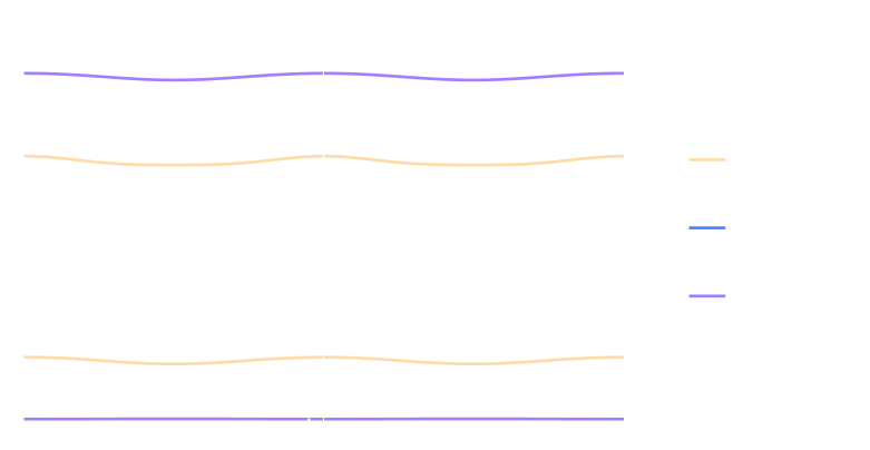
We now show by numerical experiments that the expressions we obtained, though quite lengthy in the reaction-diffusion case, are indeed very good approximations of the optimal relaxation parameters, as a function of the penalization parameter $\dd$ and in the reaction case the reaction scaling $\gamma=\frac{\eps}{h^2}$. To do so, we assemble the system matrix on a uniform 64-element mesh, with Dirichlet boundary conditions, and compute numerically the spectral radii of the two-level operators using the QR method, as implemented in LAPACK 3.6.0, accessed with Python 3.5.2.6.1. Point block-Jacobi smoother for the Poisson equation
The dotted lines in Figure 13(a) are numerically computed spectral radii $\rho$ vs. relaxation parameter $\alpha$ for $\dd = 1.2$ (red), for $\dd = 1.5$ (orange) and for $\dd = 2$ (purple) for the two-level method with the point block-Jacobi smoother. We see that they all attain a minimum value giving fastest convergence, which coincides with the theoretical prediction of Theorem 5.1 marked with blue dots and a label indicating the value of $\dd$ used. We also added a theoretical blue dot for $\dd = 1$ (top right) and $\dd \rightarrow \infty$ (bottom left), and the entire theoretically predicted parametric line $\rho(\alpha_\text{opt}(\dd),\dd)$, also in blue with $\alpha_\text{opt}(\dd)$ from Theorem 5.1. We see that our theoretical result based on the typical LFA assumption of periodic boundary conditions predicts the performance with Dirichlet boundary conditions very well. One might be tempted to use large values of $\dd$ in order to have as small a spectral radius as possible, but for large $\dd$, the coarse problem is more difficult to solve because the $\dd$ is doubled as we showed in §4.3 and the condition number of the unpreconditioned coarse operator grows. It would be interesting to investigate if the capacity of this smoother to deal with large values of $\dd$ can be used to our advantage in a multigrid setting.

6.2. Cell block-Jacobi smoother for the Poisson equation
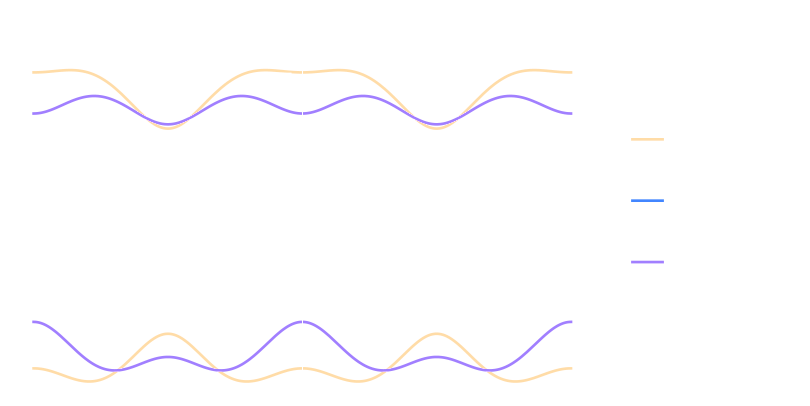
The dotted lines in Figure 13(b) are numerically computed spectral radii $\rho$ vs. relaxation parameter $\alpha$ for $\dd = 1.2$ (red), $\dd =\widetilde{\dd}_+ \approx 1.41964$ (black), $\dd =\widetilde{\dd}_- = 1.5$ (orange) and $\dd = 2$ (purple) for the two level method with the cell block-Jacobi smoother. Like for the point block-Jacobi smoother they all attain a minimum value which gives fastest convergence. With blue dots, we mark the theoretical predictions of Theorem 5.2, also for a few more values of $\dd\in\{1,1.1,1.3,4,\infty\}$. In contrast to the point block-Jacobi smoother case, the two values $\dd=1$ and $\dd=\infty$ lead to the same point on the curve at the top right, which shows that this method also deteriorates when $\dd$ becomes large. We also plot the entire theoretically predicted parametric line $\rho(\alpha_\text{opt}(\dd),\dd)$ in solid blue with $\alpha_\text{opt}(\dd)$ from Theorem 5.2 and the corresponding numerically determined one in dashed blue2. This shows that the theoretical prediction is very accurate, except for values around $\dd\approx\widetilde{\dd}_+$ where there is a small difference. We checked that this is due to the Dirichlet boundary conditions, by performing numerical experiments using periodic boundary conditions which made the results match the predicted line. We also observed that the dashed line approaches the predicted line when decreasing the mesh size. Therefore, even though Theorem 5.2 was obtained with the typical LFA assumption of periodic boundary conditions, the predictions are again very good also for the Dirichlet case. Note that in contrast to the point block-Jacobi case, where best performance is achieved for large $\dd$, for cell block-Jacobi the best performance is achieved for $\dd=\widetilde{\dd}_-$, and convergence is almost twice as fast as for point block-Jacobi with a similar value for $\dd$. Clearly, also in practice, the DG penalization parameter influences very much the performance of the two-level solver, even when using the best possible relaxation parameter.6.4. Point block-Jacobi smoother for the reaction-diffusion equation
Results for the solution of a reaction-diffusion equation using a two-level method with the point block-Jacobi smoother are shown in Figure 14(a).

Theoretically predicted parametric curves are shown for $\dd \in [1,\infty)$, while numerically computed values are shown as points for $\dd\in[1,50]$. The top right end of the curves corresponds to $\dd = 1$, while the bottom left end corresponds to $\dd \rightarrow \infty$. In blue, we can see the measured $\rho_\text{opt}$, $\alpha_\text{opt}$ as dots plotted on top of the predicted parametric curve of the same color, for $\gamma = 16$. As expected, we see that a large value of $\gamma$ almost reproduces the predicted curve that we observed for the Poisson equation (c.f. Figure 13(a)). As we modify $\gamma$ and make it smaller (in orange, green, red, violet and brown, for $\gamma=2, 2^{-1}, 4^{-1}, 8^{-1}, 16^{-1}$ respectively), the parametric curve moves towards the bottom right of the figure, while keeping its shape until $\gamma \approx 7^{-1}$ where it features a point with discontinuous derivative. Keeping in mind that the rightmost end of each curve corresponds to $\dd = 1$ and the leftmost end corresponds to $\dd \rightarrow \infty$, we observe that for any finite value of $\gamma$ the method is robust for any value of $\dd$, i.e. the convergence factor remains bounded away from 1. Large values of $\gamma$ require underrelaxation, and small values overrelaxation, and in between there are $\gamma$ values that require both overrelaxation for small $\dd$ and underrelaxation for large $\dd$ to be optimal. When $\gamma$ is very small, the regime becomes insensitive to the values of $\dd$, which is expected since all the terms in the bilinear form that describe derivatives are negligible in comparison to the reaction term and even at very large values of $\dd$, the point block-Jacobi smoother can neutralize the operator's dependency on $\dd$; see also the bottom curve in Figure 9 on the right.

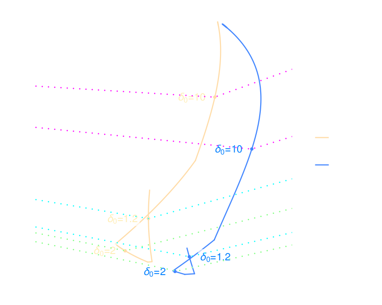
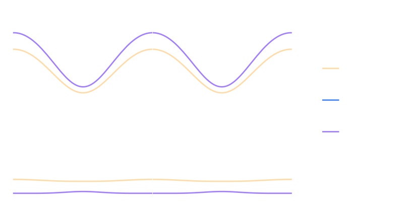
Figure 15(b) shows experiments for a range of relaxation parameters, in order to illustrate that when using the optimal relaxation, the spectral radius falls on the line of predicted values. Each dot on the v-shaped dotted line is an experiment performed for a different $\alpha$. The predicted optimal point on the solid line is indicated with a label.
Cell block-Jacobi smoother for the reaction-diffusion equation
Results for the solution of a reaction-diffusion equation using a two-level method with the cell block-Jacobi smoother are shown in Figure 14(b). Theoretically predicted parametric curves are shown for $\dd \in [1,\infty)$, while numerically computed values are shown as dashed lines for $\dd\in[1,50]$. All the curves end at $\rho_\text{opt}=1$, $\alpha_\text{opt}=1$, while they begin at smaller values of $\rho_\text{opt}$ for smaller values of $\gamma$. Once again in blue, we show the measured $\rho_\text{opt}$, $\alpha_\text{opt}$ with a dashed line, and the predicted value as a solid line, for $\gamma=16$. Such a large value of $\gamma$ is almost equivalent to the Poisson equation and the shapes of the curves of Figure 13(b) are reproduced. When we set $\gamma$ to smaller values (in orange, green, red, violet and brown, for $\gamma=2, 2^{-1}, 4^{-1}, 8^{-1}, 16^{-1}$ respectively), we see that convergence rapidly improves for values of $\dd$ that are order one, including $\dd = 1$, represented as the beginning of the curve that moves down and to the right of the figure. For moderate values of $\dd$, very small values of $\gamma$ will even result in an exact solver with the smoother alone. Convergence however still deteriorates as $\dd \rightarrow \infty$, since, unlike the point block-Jacobi smoother, the cell block-Jacobi smoother cannot neutralize the operator’s dependency on $\dd$ for $\dd$ large. The measured results (dashed) and theoretically predicted ones (solid) show very good agreement. Also, we see that small values of $\gamma$ can require overrelaxation when $\dd$ becomes large.
Figure 15(b) shows experiments for a range of relaxation parameters, in order to illustrate that when using the optimal relaxation, the spectral radius falls on the line of predicted values. Each dot on the v-shaped dotted line is an experiment performed for a different $\alpha$. The predicted optimal point on the solid line is indicated with a label.
6.5. Higher dimensions, different geometries and further research
We now test our closed form optimized relaxation parameters from the 1D analysis in higher dimensions and on geometries and meshes that go far beyond a simple tensor product generalization. To that end, we use the deal.II finite element library [1]. We show in Figure 16 a set of comparisons of the optimality of our closed form optimized relaxation parameters for the Poisson problem, using cell block-Jacobi smoothers. In each case, we show the mesh used and a comparison between the unrelaxed method, the relaxation of $2/3$ coming from the smoothing analysis alone, the one predicted by Theorem 5.2, and the numerically best performing one, which we obtained by running the code for many parameters and then taking the best performing one. The closeness between our closed form optimized parameters from the 1D analysis and the numerically best working one in higher dimensions is clear evidence that the seminal quote from P. W. Hemker in footnote 1 is more than justified.
In principle, it would be possible to extend our analysis to the case of tensor product meshes in 2D (and 3D), but this would pose important technical difficulties: in Section 4, we have seen that considering the complete 2-level error operator necessitates analyzing a $4\times 4$ matrix instead of a $2\times 2$ matrix needed for the smoothing analysis alone. For a tensor product grid in 2D, the error operator of the complete 2-level analysis would be $16 \times 16$, and a direct analysis like the one we performed in 1D would require finding exact expressions, depending on the coefficients, of polynomials of degree 16. Such difficulties have been faced by D. Le Roux et al., for specific wave propagation applications [24], and they require, when possible at all, a very careful algebraic analysis and general understanding of the tensor interactions. To the best of our knowledge, for higher dimensions, the community has turned to the numerical study of the resulting matrices, see e.g. [17, 16, 6, 20, 9] and references therein, which can not give the same depth as an analytical study. Some generalizations that tackle higher dimensions and different boundary conditions can be found in [29].
The advantage of our approach is that we can see the interactions between different components in a very clear way in 1D, and thus achieve deeper insight into the functioning of the numerical method in 1D. Furthermore, our numerical experiments in higher dimensions show that the 1D results are still giving close to optimal relaxation parameters, even on non-tensor and irregular meshes, which indicates that our 1D analysis captures fundamental diffusion and singularly perturbed reaction diffusion behavior of the underlying operator, not just in 1D and for tensor product meshes. A further illustration of the interest of our detailed 1D analysis is our publication [14] showing that the optimization can be carried as far as to obtain an exact solver from an iterative one, with exact analytical expressions for the relaxation parameters involved.
The complexity of the analytical expressions found in our 2-level analysis not withstanding, we managed, based on the results in the present manuscript, to obtain analytical expressions for finite difference stencils in 2D and 3D by using different, red/black decompositions, establishing a link with cyclic reduction. The work is however extensive and will appear elsewhere.
7. Conclusion
We optimized the relaxation parameter in two-level iterative methods for solving symmetric interior penalty discontinuous Galerkin discretized Poisson and reaction-diffusion equations using a cell block-Jacobi and a point block-Jacobi smoother. Our optimization for the complete two-level process shows that the cell block-Jacobi smoother leads to a more effective two-level method for moderate sizes of the penalization parameter, while the point block-Jacobi smoother is superior for large penalization parameters. Our analysis also reveals that the penalization parameter in SIPG should not only be chosen large enough such that the DG method converges, but it can be chosen to optimize the performance of the associated iterative two-level solver. A good choice can lead to an iterative solver that converges an order of magnitude faster than other choices, and this even using the best possible relaxation parameter in the smoother. While we performed our analysis in 1D, our numerical experiments in higher dimensions on irregular domains with irregular meshes clearly show that our closed form optimized relaxation parameters work very well also in these situations, with very close to best possible performance of the SIPG two level method.1. In 1D this is simply a This is motivated by the seminal work of P. W. Hemker [19] who stated: "we study the one-dimensional equation, since this can be considered as an essential building block for the higher dimensional case where we use tensor product polynomials". We test however our analytical results also in higher dimensions and on meshes which are not tensor products, see Subsection 6.5. ↩
2. The value $\dd=p(p+1)$ is used for example in the deal.II Finite Element Library [1] we will use in Subsection 6.5. ↩
3. We did not plot this dashed line for the point block-Jacobi smoother case in Figure 13(a), since it would not have been visible under the predicted line. ↩
Bibliography
[1] Paola F. Antonietti, Marco Sarti, and Marco Verani. Multigrid algorithms for hp-discontinuous Galerkin discretizations of elliptic problems. SIAM J. on Numer. Anal., 53(1):598–618, 2015.
[1] Arndt, D., Bangerth, W., Blais, B., Fehling, M., Gassmöller, R., Heister, T., Heltai, L., Köcher, U., Kronbichler, M., Maier, M., Munch, P., Pelteret, J.P., Proell, S., Simon, K., Turcksin, B., Wells, D., Zhang, J.: The deal.II library, version 9.3. Journal of Numerical Mathematics (2021, accepted for publication). URL https://dealii.org/deal93-preprint. pdf
[2] Arnold, D.N.: An interior penalty finite element method with discontinuous elements. SIAM J. Numer. Anal. 19(4), 742–760 (1982). DOI 10.1137/0719052
[3] Arnold, D.N., Brezzi, F., Cockburn, B., Marini, L.: Unified analysis of discontinuous Galerkin methods for elliptic problems. SIAM J. Numer. Anal. 39(5), 1749–1779 (2002)
[4] Baker, G.A.: Finite element methods for elliptic equations using nonconforming elements. Math. Comp. 137(31), 45–59 (1977)
[5] Becherer, D., Schweizer, M.: Classical solutions to reaction-diffusion systems for hedging problems with interacting itô and point processes. The Annals of Applied Probability 2(15), 1111–1144 (2005)
[6] Bolten, M., Rittich, H.: Fourier analysis of periodic stencils in multigrid methods. SIAM Journal on Scientific Computing 40(3), A1642–A1668 (2018). DOI 10.1137/16M1073959. URL https://doi.org/10.1137/16M1073959
[7] Brandt, A.: Multi-level adaptive solutions to boundary-value problems. Mathematics of Com- putation 31(138), 333–390 (1977). URL http://www.jstor.org/stable/2006422
[8] Brandt, A.: Rigorous quantitative analysis of multigrid. i. constant coefficients two-level cycle with L2 -norm. SIAM J. Numer. Anal. 6(31), 1695–1730 (1994). DOI 10.1137/0731087
[9] Brown, J., He, Y., MacLachlan, S.: Local fourier analysis of balancing domain decomposition by constraints algorithms. SIAM Journal on Scientific Computing 41(5), S346–S369 (2019). DOI 10.1137/18M1191373. URL https://doi.org/10.1137/18M1191373
[10] Dautray, R., Lions, J.L.: Mathematical analysis and numerical methods for science and tech- nology. Volume 2. , Functional and Variational Methods. Springer-Verlag, Berlin Heidelberg New York London Paris Tokyo (1985)
[11] Dryja, M., Krzyżanowski, P.: A massively parallel nonoverlapping additive Schwarz method for discontinuous Galerkin discretization of elliptic problems. Numerische Mathematik 132(2), 347–367 (2016). DOI 10.1007/s00211-015-0718-5
[12] Feng, X., Karakashian, O.: Two-level non-overlapping Schwarz methods for a discontinuous Galerkin method. SIAM J. Numer. Anal. 39(4), 1343–1365 (2001)
[13] Fife, P.C.: Mathematical Aspects of Reacting and Diffusing Systems. Springer Verlag Berlin Heidelberg New York (1979). DOI 10.1007/978-3-642.93111-6
[14] Gander, M.J., Lucero Lorca, J.P.: Should multilevel methods for discontinuous galerkin dis- cretizations use discontinuous interpolation operators? In: S.C. Brenner, E. Chung, A. Kla- wonn, F. Kwok, J. Xu, J. Zou (eds.) Domain Decomposition Methods in Science and Engi- neering XXVI, pp. 273–280. Springer International Publishing, Cham (2022)
[15] Gie, G., Hamouda, M., Jung, C., Temam, R.: Singular Perturbations and Boundary Layers. Applied Mathematical Sciences. Springer International Publishing (2018). URL https:// books.google.ch/books?id=d2V7DwAAQBAJ
[16] He, Y., MacLachlan, S.: Two-level fourier analysis of multigrid for higher-order finite- element discretizations of the laplacian. Numerical Linear Algebra with Applications 27(3), e2285 (2020). DOI https://doi.org/10.1002/nla.2285. URL https://onlinelibrary.wiley. com/doi/abs/10.1002/nla.2285
[17] He, Y., Rhebergen, S., Sterck, H.D.: Local fourier analysis of multigrid for hybridized and embedded discontinuous galerkin methods. SIAM Journal on Scientific Computing 43(5), S612–S636 (2021). DOI 10.1137/20M1346985. URL https://doi.org/10.1137/20M1346985
[18] Hemker, P., Hoffmann, W., van Raalte, M.: Two-level fourier analysis of a multigrid approach for discontinuous Galerkin discretization. SIAM Journal on Scientific Computing 3(25), 1018– 1041 (2003)
[19] Hemker, P.W., Hoffmann, W., van Raalte, M.H.: Fourier two-level analysis for discontinuous Galerkin discretization with linear elements. Numerical Linear Algebra with Applications 5 – 6(11), 473–491 (2004)
[20] Kahl, K., Kintscher, N.: Automated local Fourier analysis (aLFA). BIT Numerical Mathe- matics 60, 1572–9125 (2020). DOI 10.1007/s10543-019-00797-w
[21] Kanschat, G., Lucero Lorca, J.P.: A weakly penalized discontinuous Galerkin method for radiation in dense, scattering media. CMAM 16(4), 563–577 (2016). DOI 10.1515/ cmam-2016-0023
[22] Karakashian, O., Collins, C.: Two-level additive Schwarz methods for discontinuous Galerkin approximations of second-order elliptic problems. IMA Journal of Numerical Analysis 37, 1800–1830 (2017). DOI 10.1093/imanum/drw061
[23] Kopteva, N., O’Riordan, E.: Shishkin meshes in the numerical solution of singularly perturbed differential equations. International Journal of Numerical Analysis and Modeling 7 (2010)
[24] Le Roux, D.Y., Eldred, C., Taylor, M.A.: Fourier analyses of high-order continuous and dis- continuous galerkin methods. SIAM Journal on Numerical Analysis 58(3), 1845–1866 (2020). DOI 10.1137/19M1289595. URL https://doi.org/10.1137/19M1289595
[25] Lew, A.J., Buscaglia, G.C.: A discontinuous-Galerkin-based immersed boundary method. International Journal for Numerical Methods in Engineering 76(4), 427–454 (2008). DOI 10.1002/nme.2312. URL https://onlinelibrary.wiley.com/doi/abs/10.1002/nme.2312
[26] Lucero Lorca, J.P., Kanschat, G.: Multilevel Schwarz preconditioners for singularly perturbed symmetric reaction-diffusion systems. Electron. Trans. Numer. Anal. 54, 89–107 (2021). DOI 10.1553/etna_vol54s89
[27] Manteuffel, T.A., Ressel, K.J.: Least-squares finite-element solution of the neutron transport equation in diffusive regimes. SIAM J. Numer. Anal. 35(2), 806–835 (1998)
[28] Nitsche, J.: Über ein Variationsprinzip zur Lösung von Dirichlet-Problemen bei der Verwen- dung von Teilräumen, die keinen Randbedingungen unterworfen sind. Abh. Math. Sem. Univ. Hamburg 36, 9–15 (1971)
[29] Rodrigo CarmenGaspar, F.J., Zikatanov, L.T.: On the validity of the local fourier anal- ysis. Journal of Computational Mathematics 37(3), 340–348 (2018). DOI https://doi.org/ 10.4208/jcm.1803-m2017-0294. URL http://global-sci.org/intro/article_detail/jcm/ 12725.html
[30] Smoller, J.: Shock Waves and Reaction–Diffusion Equations. No. 258 in XXI, 581 S., 162 Abb., DM 128. Berlin, Heidelberg, New York, Springer – Verlag (1983)
[31] van der Vegt, J., Rhebergen, S.: hp-multigrid as smoother algorithm for higher or- der discontinuous galerkin discretizations of advection dominated flows: Part i. mul- tilevel analysis. Journal of Computational Physics 231(22), 7537–7563 (2012). DOI https://doi.org/10.1016/j.jcp.2012.05.038. URL https://www.sciencedirect.com/science/ article/pii/S0021999112003129
[32] van der Vegt, J., Rhebergen, S.: Hp-multigrid as smoother algorithm for higher order dis- continuous galerkin discretizations of advection dominated flows. part ii: Optimization of the runge–kutta smoother. Journal of Computational Physics 231(22), 7564–7583 (2012). DOI https://doi.org/10.1016/j.jcp.2012.05.037. URL https://www.sciencedirect.com/science/ article/pii/S0021999112003117
[33] Wheeler, M.F.: An elliptic collocation finite element method with interior penalties. SIAM J. Numer. Anal. 39(15(1)), 152–161 (1978)
[34] Zhou, Y.: Fourier Analysis and Local Fourier Analysis for Multigrid Methods. Master’s thesis, Johannes Kepler Universität Linz (2009)